
Flow through multiple layers
Storyboard 
Once the hydraulic resistance and conductivity have been calculated, it becomes possible to model a multi-layer soil system. To achieve this, it is essential to compute the total resistance and conductivity and, after establishing the overall flow, to determine the partial flows (in the case of parallel layers) or the pressure drop in each layer (in the case of series layers).
ID:(371, 0)
Hydraulic resistance of elements in series
Image
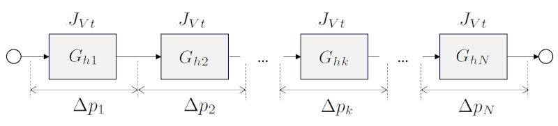
In the case of a sum where the elements are connected in series, the total hydraulic resistance of the system is calculated by summing the individual resistances of each element.

One way to model a tube with varying cross-section is to divide it into sections with constant radius and then sum the hydraulic resistances in series. Suppose we have a series of the hydraulic resistance in a network ($R_{hk}$), which depends on the viscosity ($\eta$), the cylinder k radio ($R_k$), and the tube k length ($\Delta L_k$) via the following equation:
| $ R_h =\displaystyle\frac{8 \eta | \Delta L | }{ \pi R ^4}$ |
In each segment, there will be a pressure difference in a network ($\Delta p_k$) with the hydraulic resistance in a network ($R_{hk}$) and the volume flow ($J_V$) to which Darcy's Law is applied:
| $ \Delta p = R_h J_V $ |
the total pressure difference ($\Delta p_t$) will be equal to the sum of the individual ERROR:10132,0:
| $ \Delta p_t =\displaystyle\sum_k \Delta p_k $ |
therefore,
$\Delta p_t=\displaystyle\sum_k \Delta p_k=\displaystyle\sum_k (R_{hk}J_V)=\left(\displaystyle\sum_k R_{hk}\right)J_V\equiv R_{st}J_V$
Thus, the system can be modeled as a single conduit with the hydraulic resistance calculated as the sum of the individual components:
| $ R_{st} =\displaystyle\sum_k R_{hk} $ |
ID:(3630, 0)
Hydraulic conductance of elements in series
Note
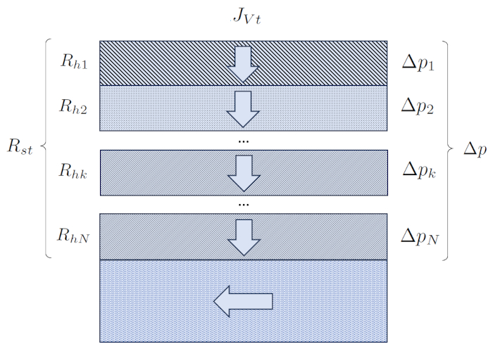
In the case of a sum where the elements are connected in series, the total hydraulic conductance of the system is calculated by adding the individual hydraulic conductances of each element.
the total hydraulic resistance in series ($R_{st}$), along with the hydraulic resistance in a network ($R_{hk}$), in
| $ R_{st} =\displaystyle\sum_k R_{hk} $ |
and along with the hydraulic conductance in a network ($G_{hk}$) and the equation
| $ R_h = \displaystyle\frac{1}{ G_h }$ |
leads to the total Series Hydraulic Conductance ($G_{st}$) can be calculated with:
| $\displaystyle\frac{1}{ G_{st} }=\displaystyle\sum_k\displaystyle\frac{1}{ G_{hk} }$ |
$\Delta p_k = \displaystyle\frac{J_{Vk}}{K_{hk}}$
So, the sum of the inverse of the hydraulic conductance in a network ($G_{hk}$) will be equal to the inverse of the total Series Hydraulic Conductance ($G_{st}$).
ID:(11067, 0)
Flow through serial soil layers
Quote
A situation in the soil where the elements are connected in series occurs when water infiltrates vertically through several layers, eventually ending up in the water table. In this case, the column Section ($S$) remains constant, while each layer has a different width that acts as the width of the kth layer ($L_k$).
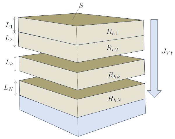
In this scenario, hydraulic resistances are directly summed, and their values depend on the type of soil, and therefore, on the hydraulic conductivity in the kth layer ($K_{sk}$) and the width of the kth layer ($L_k$).
ID:(936, 0)
Hydraulic resistance of elements in parallel
Exercise
In the case of a sum where the elements are connected in parallel, the total hydraulic resistance of the system is calculated by adding the individual resistances of each element.
the parallel total hydraulic conductance ($G_{pt}$) combined with the hydraulic conductance in a network ($G_{hk}$) in
| $ G_{pt} =\displaystyle\sum_k G_{hk} $ |
and along with the hydraulic resistance in a network ($R_{hk}$) and the equation
| $ R_h = \displaystyle\frac{1}{ G_h }$ |
leads to the total hydraulic resistance in parallel ($R_{pt}$) via
| $\displaystyle\frac{1}{ R_{pt} }=\sum_k\displaystyle\frac{1}{ R_{hk} }$ |
ID:(11068, 0)
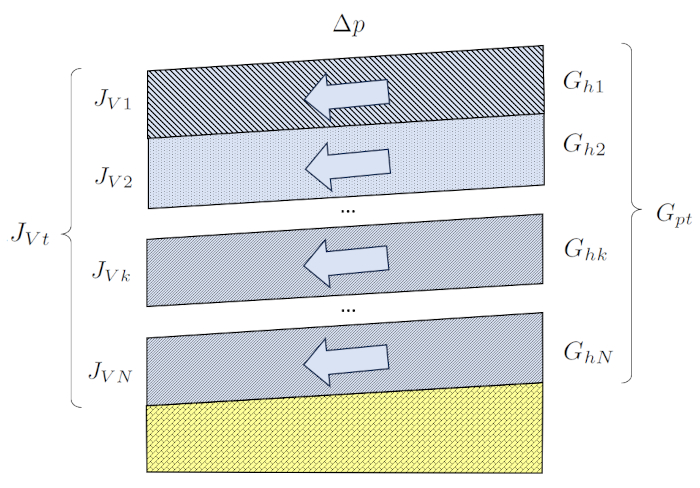
Hydraulic conductance of elements in parallel
Equation
En el caso de una suma en la que los elementos están conectados en paralelo, la conductancia hidráulica total del sistema se calcula sumando las conductancias individuales de cada elemento.
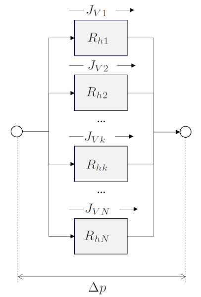
With the total flow ($J_{Vt}$) being equal to the volume flow in a network ($J_{Vk}$):
| $ J_{Vt} =\displaystyle\sum_k J_{Vk} $ |
and with the pressure difference ($\Delta p$) and the hydraulic conductance in a network ($G_{hk}$), along with the equation
| $ J_V = G_h \Delta p $ |
for each element, it leads us to the conclusion that with the parallel total hydraulic conductance ($G_{pt}$),
$J_{Vt}=\displaystyle\sum_k J_{Vk} = \displaystyle\sum_k G_{hk}\Delta p = G_{pt}\Delta p$
we have
| $ G_{pt} =\displaystyle\sum_k G_{hk} $ |
ID:(12800, 0)
Flow through parallel soil layers
Script
A situation in the soil where the elements are connected in parallel occurs when water flows through different layers in parallel. If the layers have a slope, a pressure difference is generated. If the layers have a similar thickness, the pressure difference will be the same in all layers. In this case, the sample length ($\Delta L$) is constant, while each layer has a different the section of the kth layer ($S_k$).
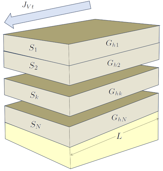
In this situation, hydraulic conductivities are directly summed, and their values depend on the type of soil, and therefore, on the hydraulic conductivity in the kth layer ($K_{sk}$) and the section of the kth layer ($S_k$).
ID:(4373, 0)
Flow through multiple layers
Storyboard
Once the hydraulic resistance and conductivity have been calculated, it becomes possible to model a multi-layer soil system. To achieve this, it is essential to compute the total resistance and conductivity and, after establishing the overall flow, to determine the partial flows (in the case of parallel layers) or the pressure drop in each layer (in the case of series layers).
Variables
Calculations
Calculations
Equations
The volume flow ($J_V$) can be calculated from the hydraulic conductance ($G_h$) and the pressure difference ($\Delta p$) using the following equation:
Furthermore, using the relationship for the hydraulic resistance ($R_h$):
results in:
One way to model a tube with varying cross-section is to divide it into sections with constant radius and then sum the hydraulic resistances in series. Suppose we have a series of the hydraulic resistance in a network ($R_{hk}$), which depends on the viscosity ($\eta$), the cylinder k radio ($R_k$), and the tube k length ($\Delta L_k$) via the following equation:
In each segment, there will be a pressure difference in a network ($\Delta p_k$) with the hydraulic resistance in a network ($R_{hk}$) and the volume flow ($J_V$) to which Darcy's Law is applied:
the total pressure difference ($\Delta p_t$) will be equal to the sum of the individual ERROR:10132,0:
therefore,
$\Delta p_t=\displaystyle\sum_k \Delta p_k=\displaystyle\sum_k (R_{hk}J_V)=\left(\displaystyle\sum_k R_{hk}\right)J_V\equiv R_{st}J_V$
Thus, the system can be modeled as a single conduit with the hydraulic resistance calculated as the sum of the individual components:
The parallel total hydraulic conductance ($G_{pt}$) combined with the hydraulic conductance in a network ($G_{hk}$) in
and along with the hydraulic resistance in a network ($R_{hk}$) and the equation
leads to the total hydraulic resistance in parallel ($R_{pt}$) via
The total hydraulic resistance in series ($R_{st}$), along with the hydraulic resistance in a network ($R_{hk}$), in
and along with the hydraulic conductance in a network ($G_{hk}$) and the equation
leads to the total Series Hydraulic Conductance ($G_{st}$) can be calculated with:
With the total flow ($J_{Vt}$) being equal to the volume flow in a network ($J_{Vk}$):
and with the pressure difference ($\Delta p$) and the hydraulic conductance in a network ($G_{hk}$), along with the equation
for each element, it leads us to the conclusion that with the parallel total hydraulic conductance ($G_{pt}$),
$J_{Vt}=\displaystyle\sum_k J_{Vk} = \displaystyle\sum_k G_{hk}\Delta p = G_{pt}\Delta p$
we have
Since the flux density ($j_s$) is related to the radius of a generic grain ($r_0$), the porosity ($f$), the liquid density ($\rho_w$), the gravitational Acceleration ($g$), the viscosity ($\eta$), the generic own porosity ($q_0$), the height difference ($\Delta h$), and the sample length ($\Delta L$) through the equation:
We can define a factor that we'll call the hydraulic conductivity ($K_s$) as follows:
This factor encompasses all the elements related to the properties of both the soil and the liquid that flows through it.
As the hydraulic resistance ($R_h$) is associated with the hydraulic conductivity ($K_s$), the liquid density ($\rho_w$), the gravitational Acceleration ($g$), the column Section ($S$), and the sample length ($\Delta L$), it is expressed as
And the relationship for the hydraulic conductance ($G_h$)
leads to
With Darcy's law, where the pressure difference ($\Delta p$) equals the hydraulic resistance ($R_h$) and the total flow ($J_{Vt}$):
Thus, with the equation for the soil with the section Flow ($S$), the radius of a generic grain ($r_0$), the viscosity ($\eta$), the generic own porosity ($q_0$), the porosity ($f$), the pressure difference ($\Delta p$), and the sample length ($\Delta L$):
Therefore, the hydraulic resistance ($R_h$) is:
Calculating the hydraulic resistance ($R_h$) using the viscosity ($\eta$), the generic own porosity ($q_0$), the radius of a generic grain ($r_0$), the porosity ($f$), the sample length ($\Delta L$), and the column Section ($S$) through
and utilizing the expression for the hydraulic conductivity ($K_s$)
is obtained after replacing the common factors
If we examine the Hagen-Poiseuille law, which allows us to calculate the volume flow ($J_V$) from the tube radius ($R$), the viscosity ($\eta$), the tube length ($\Delta L$), and the pressure difference ($\Delta p$):
we can introduce the hydraulic conductance ($G_h$), defined in terms of the tube length ($\Delta L$), the tube radius ($R$), and the viscosity ($\eta$), as follows:
to arrive at:
Examples
In the case of a sum where the elements are connected in series, the total hydraulic resistance of the system is calculated by summing the individual resistances of each element.
One way to model a tube with varying cross-section is to divide it into sections with constant radius and then sum the hydraulic resistances in series. Suppose we have a series of the hydraulic resistance in a network ($R_{hk}$), which depends on the viscosity ($\eta$), the cylinder k radio ($R_k$), and the tube k length ($\Delta L_k$) via the following equation:
In each segment, there will be a pressure difference in a network ($\Delta p_k$) with the hydraulic resistance in a network ($R_{hk}$) and the volume flow ($J_V$) to which Darcy's Law is applied:
the total pressure difference ($\Delta p_t$) will be equal to the sum of the individual ERROR:10132,0:
therefore,
$\Delta p_t=\displaystyle\sum_k \Delta p_k=\displaystyle\sum_k (R_{hk}J_V)=\left(\displaystyle\sum_k R_{hk}\right)J_V\equiv R_{st}J_V$
Thus, the system can be modeled as a single conduit with the hydraulic resistance calculated as the sum of the individual components:
In the case of a sum where the elements are connected in series, the total hydraulic conductance of the system is calculated by adding the individual hydraulic conductances of each element.
the total hydraulic resistance in series ($R_{st}$), along with the hydraulic resistance in a network ($R_{hk}$), in
and along with the hydraulic conductance in a network ($G_{hk}$) and the equation
leads to the total Series Hydraulic Conductance ($G_{st}$) can be calculated with:
$\Delta p_k = \displaystyle\frac{J_{Vk}}{K_{hk}}$
So, the sum of the inverse of the hydraulic conductance in a network ($G_{hk}$) will be equal to the inverse of the total Series Hydraulic Conductance ($G_{st}$).
A situation in the soil where the elements are connected in series occurs when water infiltrates vertically through several layers, eventually ending up in the water table. In this case, the column Section ($S$) remains constant, while each layer has a different width that acts as the width of the kth layer ($L_k$).
In this scenario, hydraulic resistances are directly summed, and their values depend on the type of soil, and therefore, on the hydraulic conductivity in the kth layer ($K_{sk}$) and the width of the kth layer ($L_k$).
One efficient way to model a tube with varying cross-sections is to divide it into sections with constant radii and then sum the hydraulic resistances in series. Suppose we have a series of elements the hydraulic resistance in a network ($R_{hk}$), whose resistance depends on the viscosity ($\eta$), the cylinder k radio ($R_k$), and the tube k length ($\Delta L_k$), according to the following equation:
In each element, we consider a pressure difference in a network ($\Delta p_k$) along with the hydraulic resistance in a network ($R_{hk}$) and the volumetric flow rate the volume flow ($J_V$), where Darcy's law is applied:
The total resistance of the system, the flujo de Volumen Total ($J_{Vt}$), is equal to the sum of the individual hydraulic resistances ERROR:10133,0 of each section:
Thus, we have:
$J_{Vt}=\displaystyle\sum_k \Delta J_{Vk}=\displaystyle\sum_k \displaystyle\frac{\Delta p_k}{R_{hk}}=\left(\displaystyle\sum_k \displaystyle\frac{1}{R_{hk}}\right)\Delta p\equiv \displaystyle\frac{1}{R_{pt}}J_V$
Therefore, the system can be modeled as a single conduit with a total hydraulic resistance calculated by summing the individual components:
The flujo de Volumen Total ($J_{Vt}$) represents the total sum of the individual contributions from the volume flow 1 ($J_{V1}$) and the volume flow 2 ($J_{V2}$), from the elements connected in parallel:
A situation in the soil where the elements are connected in parallel occurs when water flows through different layers in parallel. If the layers have a slope, a pressure difference is generated. If the layers have a similar thickness, the pressure difference will be the same in all layers. In this case, the sample length ($\Delta L$) is constant, while each layer has a different the section of the kth layer ($S_k$).
In this situation, hydraulic conductivities are directly summed, and their values depend on the type of soil, and therefore, on the hydraulic conductivity in the kth layer ($K_{sk}$) and the section of the kth layer ($S_k$).
The flow of liquid in a porous medium such as soil is measured using the variable the flux density ($j_s$), which represents the average velocity at which the liquid moves through it. When modeling the soil and how the liquid passes through it, it is found that this process is influenced by factors such as the porosity ($f$) and the radius of a generic grain ($r_0$), which, when greater, facilitate the flow, whereas the viscosity ($\eta$) hinders passage through capillaries, reducing the flow velocity.
The modeling eventually incorporates what we will call the hydraulic conductivity ($K_s$), a variable that depends on the interactions between the radius of a generic grain ($r_0$), the porosity ($f$), the liquid density ($\rho_w$), the gravitational Acceleration ($g$), the viscosity ($\eta$), and the generic own porosity ($q_0$):
the hydraulic conductivity ($K_s$) expresses how easily the liquid is conducted through the porous medium. In fact, the hydraulic conductivity ($K_s$) increases with the porosity ($f$) and the radius of a generic grain ($r_0$), and decreases with the generic own porosity ($q_0$) and the viscosity ($\eta$).
As the total flow ($J_{Vt}$) is related to the radius of a generic grain ($r_0$), the porosity ($f$), the liquid density ($\rho_w$), the gravitational Acceleration ($g$), the viscosity ($\eta$), the generic own porosity ($q_0$), the column Section ($S$), and the sample length ($\Delta L$), it is equal to:
Therefore, the hydraulic conductance ($G_h$) is equal to:
In the context of electrical resistance, there exists its inverse, known as electrical conductance. Similarly, what would be the hydraulic conductance ($G_h$) can be defined in terms of the hydraulic resistance ($R_h$) through the expression:
Calculating the hydraulic resistance ($R_h$) with the viscosity ($\eta$), the generic own porosity ($q_0$), the radius of a generic grain ($r_0$), the porosity ($f$), the sample length ($\Delta L$), and the column Section ($S$) using
which can be rewritten using the expression for the hydraulic conductivity ($K_s$) with the liquid density ($\rho_w$) and the gravitational Acceleration ($g$), resulting in
As the hydraulic resistance ($R_h$) is related to the hydraulic conductivity ($K_s$), the liquid density ($\rho_w$), the gravitational Acceleration ($g$), the column Section ($S$), and the sample length ($\Delta L$), it is expressed as
Since the hydraulic conductance ($G_h$) is the inverse of the hydraulic resistance ($R_h$), we can conclude that
The total pressure difference ($\Delta p_t$) in relation to the various ERROR:10132,0, leading us to the following conclusion:
Darcy rewrites the Hagen Poiseuille equation so that the pressure difference ($\Delta p$) is equal to the hydraulic resistance ($R_h$) times the volume flow ($J_V$):
When there are multiple hydraulic resistances connected in series, we can calculate the total hydraulic resistance in series ($R_{st}$) by summing the hydraulic resistance in a network ($R_{hk}$), as expressed in the following formula:
In the case of hydraulic resistances in series, the inverse of the total Series Hydraulic Conductance ($G_{st}$) is calculated by summing the inverses of each the hydraulic conductance in a network ($G_{hk}$):
Since each the hydraulic resistance of the kth layer ($R_{sk}$), which is a function of the liquid density ($\rho_w$), the gravitational Acceleration ($g$), the layer section ($S$), the width of the kth layer ($L_k$), and the hydraulic conductivity in the kth layer ($K_{sk}$), is
it follows that the total hydraulic resistance in series ($R_{st}$) is
The sum of soil layers in parallel, denoted as the total flow ($J_{Vt}$), is equal to the sum of the volume flow in a network ($J_{Vk}$):
With the introduction of the hydraulic conductance ($G_h$), we can rewrite the Hagen-Poiseuille equation with the pressure difference ($\Delta p$) and the volume flow ($J_V$) using the following equation:
The parallel total hydraulic conductance ($G_{pt}$) is calculated with the sum of the hydraulic conductance in a network ($G_{hk}$):
The total hydraulic resistance in parallel ($R_{pt}$) can be calculated as the inverse of the sum of the hydraulic resistance in a network ($R_{hk}$):
Considering that each the hydraulic conductance in a network ($G_{hk}$), dependent on the liquid density ($\rho_w$), the gravitational Acceleration ($g$), the soil layer length ($L$), the section of the kth layer ($S_k$), and the hydraulic conductivity in the kth layer ($K_{sk}$), is equal to:
Therefore, the parallel total hydraulic conductance ($G_{pt}$) is calculated as:
ID:(371, 0)