Storyboard

It is considered a column with water with a hole in its lower part. The emptying is monitored obtaining an output speed depending on the height of the column.

If the data is modeled with Bernoulli but the exit through the hole is modeled with Hagen Poiseville, which corrects the problem of the case in which it was assumed without viscosity.

>Model

ID:(1428, 0)

Iframe

>Top

ID:(15492, 0)

Description

>Top

If there is a column height ($h$) of liquid with the liquid density ($\rho_w$) under the effect of gravity, using the gravitational Acceleration ($g$), the variación de la Presión ($\Delta p$) is generated according to:

This the variación de la Presión ($\Delta p$) produces a flow through the outlet tube with the tube length ($\Delta L$), the tube radius ($R$), and the viscosity ($\eta$) of a volume flow 1 ($J_{V1}$) according to the Hagen-Poiseuille law:

Since this equation includes the section in point 2 ($S_2$), the flux density 2 ($j_{s2}$) can be calculated using:

With this, we obtain:

which corresponds to an average velocity.

To model the system, the key parameters are:

• Interior diameter of the container: 93 mm

• Interior diameter of the evacuation channel: 3.2 mm

• Length of the evacuation channel: 18 mm

The initial liquid height is 25 cm.

ID:(9870, 0)

Description

>Top

If we analyze the equation

which describes the application of Hagen-Poiseuille, we observe that the curve only matches the experimental data under the following conditions:

The velocity is low (when the column is nearly empty).

The radius of the evacuation channel must be reduced from 1.5 mm to 0.6 mm.

This shows that the flow is primarily turbulent and that only at low velocity levels is the velocity low enough for the Reynolds number to be low and the flow to be laminar.

ID:(11065, 0)

Description

>Top

If the Tracker program is used, the height of the meniscus of the column and the range of the jet can be measured. The relationship between the two is shown in the following graph:

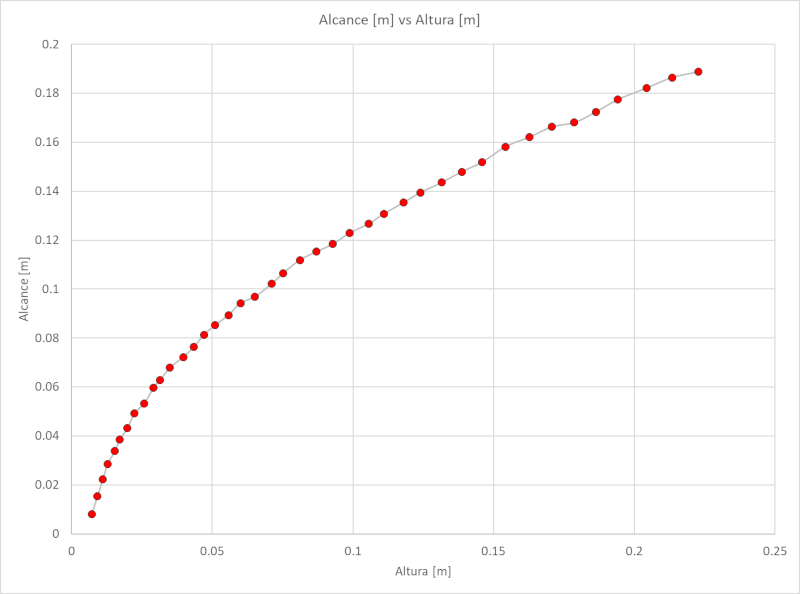
Reach [m] vs Height [m]

The recorded data, which can be downloaded as an Excel table from the following link excel table, are as follows:

Note: E indicates scientific notation (ej. 1.2E+3 = 1.2x10^3 = 1200, y 1.2E-3 = 1.2x10^-3 = 0.0012)

ID:(11062, 0)

Top

>Top

Parameters

$\tau_{hp}$

tau_hp

Characteristic time column with Hagen Pouseuille

s

$g$

g

Gravitational Acceleration

m/s^2

$\rho_w$

rho_w

Liquid density

kg/m^3

$\pi$

pi

Pi

rad

$R$

R

Tube radius

m

$\Delta p$

Dp

Variación de la Presión

Pa

$\eta$

eta

Viscosity

Pa s

Variables

$h$

h

Column height

m

$r$

r

Disc radius

m

$j_{s1}$

j_s1

Flux density 1

m/s

$j_{s2}$

j_s2

Flux density 2

m/s

$h_0$

h_0

Initial height of liquid column

m

$S_1$

S_1

Section in point 1

m^2

$S_2$

S_2

Section in point 2

m^2

$t$

t

Time

s

$\Delta t$

Dt

Time elapsed

s

$\Delta s$

Ds

Tube element

m

$\Delta L$

DL

Tube length

m

$J_{V1}$

J_V1

Volume flow 1

m^3/s

$J_{V2}$

J_V2

Volume flow 2

m^3/s

Calculations

• Alternative method
• Traditional method
• Strategy
• 2D
• 3D

Equation

Number

First, select the equation: to , then, select the variable: to

---

Calculations

Symbol

Equation

Solved

Translated

Calculations

Symbol

Equation

Solved

Translated

Variable Given Calculate Target : Equation To be used

Equations

ID:(15494, 0)

Equation

>Top, >Model

The characteristic time column with Hagen Pouseuille ($\tau_{hp}$) is calculated from the gravitational Acceleration ($g$), the liquid density ($\rho_w$), the tube length ($\Delta L$), the tube radius ($R$), the section in point 2 ($S_2$), and the viscosity ($\eta$) using:

$\tau_{hp} = \displaystyle\frac{S \Delta L}{\pi R^4}\displaystyle\frac{8 \eta}{\rho g}$

Conditions

Variables

$\tau_{hp}$

Characteristic time column with Hagen Pouseuille

$s$

10087

$g$

Gravitational Acceleration

9.8

$m/s^2$

5310

$\rho_w$

Liquid density

$kg/m^3$

5407

$\pi$

Pi

3.1415927

$rad$

5057

$S$

$S_2$

Section in point 2

$m^2$

5413

$\Delta L$

Tube length

$m$

5430

$R$

Tube radius

$m$

5417

$\eta$

Viscosity

$Pa s$

5422

Relation

ID:(14521, 0)

Equation

>Top, >Model

Given the model for the flow of a viscous liquid through a tube, and considering that the height of the column determines the pressure, we can estimate the flux density ($j_s$) as a function of the column height ($h$), using the gravitational Acceleration ($g$), the liquid density ($\rho_w$), the tube length ($\Delta L$), the tube radius ($R$), and the viscosity ($\eta$) through:

$j_{s2} = \displaystyle\frac{ \rho_w g R ^2}{8 \eta \Delta L } h$

$j_s = \displaystyle\frac{ \rho_w g R ^2}{8 \eta \Delta L } h$

Conditions

Variables

$h$

Column height

$m$

5406

$j_s$

$j_{s2}$

Flux density 2

$m/s$

10289

$g$

Gravitational Acceleration

9.8

$m/s^2$

5310

$\rho_w$

Liquid density

$kg/m^3$

5407

$\Delta L$

Tube length

$m$

5430

$R$

Tube radius

$m$

5417

$\eta$

Viscosity

$Pa s$

5422

Relation

Development

If we consider that the drainage channel presents hydraulic resistance, we can model it using the Hagen-Poiseuille equation:

$J_{V2} =-\displaystyle\frac{ \pi R ^4}{8 \eta }\displaystyle\frac{ \Delta p }{ \Delta L }$

where the pressure difference is determined by the water column:

$p = \rho_w g h$

and the velocity is obtained through the flow:

$j_s = \displaystyle\frac{ J_V }{ S }$

In this way, we obtain the relationship for calculating the velocity as a function of height:

$j_s = \displaystyle\frac{ \rho_w g R ^2}{8 \eta \Delta L } h$

ID:(11064, 0)

Equation

>Top, >Model

The column height ($h$), as a function of the time ($t$), exhibits an exponential behavior involving the initial height of liquid column ($h_0$) and the characteristic time column with Hagen Pouseuille ($\tau_{hp}$):

$h = h_0 e^{-t/\tau_{hp}}$

Conditions

Variables

$\tau_{hp}$

Characteristic time column with Hagen Pouseuille

$s$

10087

$h$

Column height

$m$

5406

$h_0$

Initial height of liquid column

$m$

10085

$t$

Time

$s$

5264

Relation

Development

If in the equation

$S \displaystyle\frac{dh}{dt} = - \displaystyle\frac{\pi R^4}{\Delta L}\displaystyle\frac{\rho g}{8 \eta} h$

the constants are replaced by

$\tau_{hp} = \displaystyle\frac{S \Delta L}{\pi R^4}\displaystyle\frac{8 \eta}{\rho g}$

we obtain the first-order linear differential equation

$\displaystyle\frac{dh}{dt}=\displaystyle\frac{1}{\tau_{hp}} h$

whose solution is

$h = h_0 e^{-t/\tau_{hp}}$

ID:(14522, 0)

Equation

>Top, >Model

One of the most basic laws in physics is the conservation of mass, which holds true throughout our macroscopic world. Only in the microscopic world does a conversion between mass and energy exist, which we will not consider in this case. In the case of a fluid, this means that the mass entering through a pipe must be equal to the mass exiting it.

If density is constant, the same applies to volume. In such cases, when we treat the flow as an incompressible fluid, it means that a given volume entering one end of the pipe must exit the other end. This can be expressed as the equality between the flow in Position 1 ($J_1$) and the flow in Position 2 ($J_2$), with the equation:

$J_{V1} = J_{V2}$

Conditions

Variables

$J_{V1}$

Volume flow 1

$m^3/s$

8478

$J_{V2}$

Volume flow 2

$m^3/s$

8479

Relation

ID:(939, 0)

Equation

>Top, >Model

The principle of continuity dictates that the flow at the first point, which is equal to the flux density 1 ($j_{s1}$) times the section in point 1 ($S_1$), must be equal to the flow at the second point, given by the flux density 2 ($j_{s2}$) times the section in point 2 ($S_2$). From this, it follows that:

$S_1 j_{s1} = S_2 j_{s2}$

Conditions

Variables

$j_{s1}$

Flux density 1

$m/s$

10288

$j_{s2}$

Flux density 2

$m/s$

10289

$S_1$

Section in point 1

$m^2$

5257

$S_2$

Section in point 2

$m^2$

5413

Relation

ID:(4350, 0)

Equation

>Top, >Model

The flux density ($j_s$) is related to the distance traveled in a time ($\Delta s$), which is the distance that the fluid travels in the time elapsed ($\Delta t$), as follows:

$j_{s1} =\displaystyle\frac{ \Delta s }{ \Delta t }$

$j_s =\displaystyle\frac{ \Delta s }{ \Delta t }$

Conditions

Variables

$j_s$

$j_{s1}$

Flux density 1

$m/s$

10288

$\Delta t$

Time elapsed

$s$

5103

$\Delta s$

Tube element

$m$

10291

Relation

ID:(4348, 0)

Equation

>Top, >Model

A flux density ($j_s$) can be expressed in terms of the volume flow ($J_V$) using the section or Area ($S$) through the following formula:

$j_{s1} = \displaystyle\frac{ J_{V1} }{ S_1 }$

$j_s = \displaystyle\frac{ J_V }{ S }$

Conditions

Variables

$j_s$

$j_{s1}$

Flux density 1

$m/s$

10288

$S$

$S_1$

Section in point 1

$m^2$

5257

$J_V$

$J_{V1}$

Volume flow 1

$m^3/s$

8478

Relation

Development

Flow is defined as the volume the volume element ($\Delta V$) divided by time the time elapsed ($\Delta t$), which is expressed in the following equation:

$J_V =\displaystyle\frac{ \Delta V }{ \Delta t }$

and the volume equals the cross-sectional area the section Tube ($S$) multiplied by the distance traveled the tube element ($\Delta s$):

$\Delta V = S \Delta s$

Since the distance traveled the tube element ($\Delta s$) per unit time the time elapsed ($\Delta t$) corresponds to the velocity, it is represented by:

$j_{s1} =\displaystyle\frac{ \Delta s }{ \Delta t }$

Thus, the flow is a flux density ($j_s$), which is calculated using:

$j_s = \displaystyle\frac{ J_V }{ S }$

ID:(4349, 1)

Equation

>Top, >Model

A flux density ($j_s$) can be expressed in terms of the volume flow ($J_V$) using the section or Area ($S$) through the following formula:

$j_{s2} = \displaystyle\frac{ J_{V2} }{ S_2 }$

$j_s = \displaystyle\frac{ J_V }{ S }$

Conditions

Variables

$j_s$

$j_{s2}$

Flux density 2

$m/s$

10289

$S$

$S_2$

Section in point 2

$m^2$

5413

$J_V$

$J_{V2}$

Volume flow 2

$m^3/s$

8479

Relation

Development

Flow is defined as the volume the volume element ($\Delta V$) divided by time the time elapsed ($\Delta t$), which is expressed in the following equation:

$J_V =\displaystyle\frac{ \Delta V }{ \Delta t }$

and the volume equals the cross-sectional area the section Tube ($S$) multiplied by the distance traveled the tube element ($\Delta s$):

$\Delta V = S \Delta s$

Since the distance traveled the tube element ($\Delta s$) per unit time the time elapsed ($\Delta t$) corresponds to the velocity, it is represented by:

$j_{s1} =\displaystyle\frac{ \Delta s }{ \Delta t }$

Thus, the flow is a flux density ($j_s$), which is calculated using:

$j_s = \displaystyle\frac{ J_V }{ S }$

ID:(4349, 2)

Equation

>Top, >Model

The volume flow ($J_V$) can be calculated with the Hagen-Poiseuille law that with the parameters the viscosity ($\eta$), the pressure difference ($\Delta p$), the tube radius ($R$) and the tube length ($\Delta L$) is:

$J_{V2} =-\displaystyle\frac{ \pi R ^4}{8 \eta }\displaystyle\frac{ \Delta p }{ \Delta L }$

$J_V =-\displaystyle\frac{ \pi R ^4}{8 \eta }\displaystyle\frac{ \Delta p }{ \Delta L }$

Conditions

Variables

$\pi$

Pi

3.1415927

$rad$

5057

$\Delta L$

Tube length

$m$

5430

$R$

Tube radius

$m$

5417

$\Delta p$

Variación de la Presión

$Pa$

6673

$\eta$

Viscosity

$Pa s$

5422

$J_V$

$J_{V2}$

Volume flow 2

$m^3/s$

8479

Relation

Development

If we consider the profile of speed on a cylinder radio ($v$) for a fluid in a cylindrical channel, where the speed on a cylinder radio ($v$) varies with respect to radius of position in a tube ($r$) according to the following expression:

$v = v_{max} \left(1-\displaystyle\frac{ r ^2}{ R ^2}\right)$

involving the tube radius ($R$) and the maximum flow rate ($v_{max}$). We can calculate the maximum flow rate ($v_{max}$) using the viscosity ($\eta$), the pressure difference ($\Delta p$), and the tube length ($\Delta L$) as follows:

$v_{max} =-\displaystyle\frac{ R ^2}{4 \eta }\displaystyle\frac{ \Delta p }{ \Delta L }$

If we integrate the velocity across the cross-section of the channel, we obtain the volume flow ($J_V$), defined as the integral of $\pi r v(r)$ with respect to radius of position in a tube ($r$) from $0$ to tube radius ($R$). This integral can be simplified as follows:

$J_V=-\displaystyle\int_0^Rdr \pi r v(r)=-\displaystyle\frac{R^2}{4\eta}\displaystyle\frac{\Delta p}{\Delta L}\displaystyle\int_0^Rdr \pi r \left(1-\displaystyle\frac{r^2}{R^2}\right)$

The integration yields the resulting Hagen-Poiseuille law:

$J_V =-\displaystyle\frac{ \pi R ^4}{8 \eta }\displaystyle\frac{ \Delta p }{ \Delta L }$

ID:(3178, 0)

Equation

>Top, >Model

The height difference, denoted by the height difference ($\Delta h$), implies that the pressure in both columns is distinct. In particular, the pressure difference ($\Delta p$) is a function of the liquid density ($\rho_w$), the gravitational Acceleration ($g$), and the height difference ($\Delta h$), as follows:

$\Delta p = \rho_w g h$

$\Delta p = \rho_w g \Delta h$

Conditions

Variables

$g$

Gravitational Acceleration

9.8

$m/s^2$

5310

$\Delta h$

$h$

Column height

$m$

5406

$\rho_w$

Liquid density

$kg/m^3$

5407

$\Delta p$

Variación de la Presión

$Pa$

6673

Relation

Development

If there is the pressure difference ($\Delta p$) between two points, as determined by the equation:

$\Delta p = p_2 - p_1$

we can utilize the water column pressure ($p$), which is defined as:

$p_t = p_0 + \rho_w g h$

This results in:

$\Delta p=p_2-p_1=p_0+\rho_wh_2g-p_0-\rho_wh_1g=\rho_w(h_2-h_1)g$

As the height difference ($\Delta h$) is:

$\Delta h = h_2 - h_1$

the pressure difference ($\Delta p$) can be expressed as:

$\Delta p = \rho_w g \Delta h$

ID:(4345, 0)

Equation

>Top, >Model

The surface of a disk ($S$) of ($$) is calculated as follows:

$S_1 = \pi r ^2$

$S = \pi r ^2$

Conditions

Variables

$r$

Disc radius

$m$

5275

$\pi$

Pi

3.1415927

$rad$

5057

$S$

$S_1$

Section in point 1

$m^2$

5257

Relation

ID:(3804, 1)

Equation

>Top, >Model

The surface of a disk ($S$) of ($$) is calculated as follows:

$S_2 = \pi R ^2$

$S = \pi r ^2$

Conditions

Variables

$r$

$R$

Tube radius

$m$

5417

$\pi$

Pi

3.1415927

$rad$

5057

$S$

$S_2$

Section in point 2

$m^2$

5413

Relation

ID:(3804, 2)