Model for Stock (RNN)
Storyboard 
The stock model takes historical segments and the value that follows them and seeks to recognize the pattern and after any sequence infer how it will continue.
Code and data
ID:(1792, 0)
Import libraries
Description 
Import the necessary libraries:
# importing the libraries
import numpy as np
import matplotlib.pyplot as plt
import pandas as pd
import warnings
warnings.filterwarnings('ignore')
ID:(13872, 0)
Load data
Description 
Load historical stock prices from google:
# load stock prices
dataset_train = pd.read_csv('stock_price_train.csv')
print(dataset_train)
Date Open High Low Close Volume
0 1/3/2012 325.25 332.83 324.97 663.59 7,380,500
1 1/4/2012 331.27 333.87 329.08 666.45 5,749,400
2 1/5/2012 329.83 330.75 326.89 657.21 6,590,300
3 1/6/2012 328.34 328.77 323.68 648.24 5,405,900
4 1/9/2012 322.04 322.29 309.46 620.76 11,688,800
... ... ... ... ... ... ...
1253 12/23/2016 790.90 792.74 787.28 789.91 623,400
1254 12/27/2016 790.68 797.86 787.66 791.55 789,100
1255 12/28/2016 793.70 794.23 783.20 785.05 1,153,800
1256 12/29/2016 783.33 785.93 778.92 782.79 744,300
1257 12/30/2016 782.75 782.78 770.41 771.82 1,770,000
[1258 rows x 6 columns]
ID:(13873, 0)
Extract opening prices
Description 
Form an arrangement with the data of the opening prices of the share:
# extract opening prices
train = dataset_train.loc[:, ['Open']].values
train
array([[325.25],
[331.27],
[329.83],
...,
[793.7 ],
[783.33],
[782.75]])
ID:(13874, 0)
Rescale values
Description 
To improve the quality of learning, the values between 0 and 1 are re-scaled:
# feature scaling
from sklearn.preprocessing import MinMaxScaler
scaler = MinMaxScaler(feature_range = (0, 1))
train_scaled = scaler.fit_transform(train)
train_scaled
array([[0.08581368],
[0.09701243],
[0.09433366],
...,
[0.95725128],
[0.93796041],
[0.93688146]])
ID:(13875, 0)
Show values
Description 
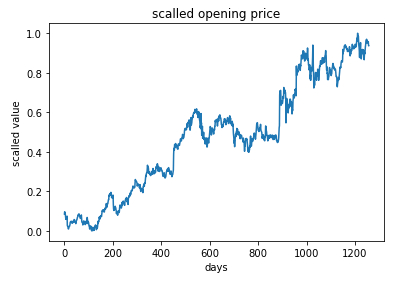
The values can be represented in time:
# show data
plt.plot(train_scaled)
plt.title('scalled opening price')
plt.xlabel('days')
plt.ylabel('scalled value')
plt.show()

ID:(13876, 0)
Create Segments
Description 
For modeling, 1208 sequences of 50 X_train values and the following y_train value are extracted:
# creating a data structure with 50 timesteps and 1 output
X_train = []
y_train = []
timesteps = 50
for i in range(timesteps, 1258):
    X_train.append(train_scaled[i-timesteps:i, 0])
    y_train.append(train_scaled[i, 0])
X_train, y_train = np.array(X_train), np.array(y_train)
ID:(13877, 0)
Re-order values
Description 
Reorder the training values train with the np.reshape function:
# reshaping
X_train = np.reshape(X_train, (X_train.shape[0], X_train.shape[1], 1))
print(X_train.shape[0],',',X_train.shape[1],',',y_train.shape[0])
print('X_train=',X_train)
print('y_train=',y_train)
1208 , 50 , 1208
X_train= [[[0.08581368]
[0.09701243]
[0.09433366]
...
[0.03675869]
[0.04486941]
[0.05065481]]
...
[[0.96569685]
[0.97510976]
[0.95966962]
...
[0.95163331]
[0.95725128]
[0.93796041]]]
y_train= [0.05214302 ... 0.93688146]
ID:(13878, 0)
Define, train and train model
Description 
The model is defined as a Sequential () sequential model, four SimpleRNN layers are added with the add function and a final single element layer . The model is structured with the compile command and then training it with the fit command:
# importing the Keras libraries and packages
from keras.models import Sequential
from keras.layers import Dense
from keras.layers import SimpleRNN
from keras.layers import Dropout

# initialising the RNN
regressor = Sequential()

# adding the first RNN layer and some Dropout regularisation
regressor.add(SimpleRNN(units = 50,activation='tanh', return_sequences = True, input_shape = (X_train.shape[1], 1)))
regressor.add(Dropout(0.2))

# adding a second RNN layer and some Dropout regularisation
regressor.add(SimpleRNN(units = 50,activation='tanh', return_sequences = True))
regressor.add(Dropout(0.2))

# adding a third RNN layer and some Dropout regularisation
regressor.add(SimpleRNN(units = 50,activation='tanh', return_sequences = True))
regressor.add(Dropout(0.2))

# adding a fourth RNN layer and some Dropout regularisation
regressor.add(SimpleRNN(units = 50))
regressor.add(Dropout(0.2))

# adding the output layer
regressor.add(Dense(units = 1))

# compiling the RNN
regressor.compile(optimizer = 'adam', loss = 'mean_squared_error')

# fitting the RNN to the Training set
regressor.fit(X_train, y_train, epochs = 100, batch_size = 32)
Epoch 1/100
38/38 [==============================] - 17s 20ms/step - loss: 0.4512
Epoch 2/100
38/38 [==============================] - 1s 19ms/step - loss: 0.2486
Epoch 3/100
38/38 [==============================] - 1s 18ms/step - loss: 0.1825
...
Epoch 98/100
38/38 [==============================] - 1s 19ms/step - loss: 0.0021
Epoch 99/100
38/38 [==============================] - 1s 19ms/step - loss: 0.0022
Epoch 100/100
38/38 [==============================] - 1s 18ms/step - loss: 0.0022
ID:(13879, 0)
Load data to evaluate
Description 
Load google stock prices for 2017 to compare to forecasted prices:
# load real stock prices (2017)
dataset_test = pd.read_csv('stock_price_test.csv')
print(dataset_test)
Date Open High Low Close Volume
0 1/3/2017 778.81 789.63 775.80 786.14 1,657,300
1 1/4/2017 788.36 791.34 783.16 786.90 1,073,000
2 1/5/2017 786.08 794.48 785.02 794.02 1,335,200
3 1/6/2017 795.26 807.90 792.20 806.15 1,640,200
4 1/9/2017 806.40 809.97 802.83 806.65 1,272,400
5 1/10/2017 807.86 809.13 803.51 804.79 1,176,800
6 1/11/2017 805.00 808.15 801.37 807.91 1,065,900
7 1/12/2017 807.14 807.39 799.17 806.36 1,353,100
8 1/13/2017 807.48 811.22 806.69 807.88 1,099,200
9 1/17/2017 807.08 807.14 800.37 804.61 1,362,100
10 1/18/2017 805.81 806.21 800.99 806.07 1,294,400
11 1/19/2017 805.12 809.48 801.80 802.17 919,300
12 1/20/2017 806.91 806.91 801.69 805.02 1,670,000
13 1/23/2017 807.25 820.87 803.74 819.31 1,963,600
14 1/24/2017 822.30 825.90 817.82 823.87 1,474,000
15 1/25/2017 829.62 835.77 825.06 835.67 1,494,500
16 1/26/2017 837.81 838.00 827.01 832.15 2,973,900
17 1/27/2017 834.71 841.95 820.44 823.31 2,965,800
18 1/30/2017 814.66 815.84 799.80 802.32 3,246,600
19 1/31/2017 796.86 801.25 790.52 796.79 2,160,600
ID:(13880, 0)
Extract opening prices to evaluate
Description 
Form an arrangement with the data of the opening prices of the stock for the evaluation:
# extract opening prices para evaluar
real_stock_price = dataset_test.loc[:, ['Open']].values
real_stock_price
array([[778.81],
[788.36],
[786.08],
[795.26],
[806.4 ],
[807.86],
[805. ],
[807.14],
[807.48],
[807.08],
[805.81],
[805.12],
[806.91],
[807.25],
[822.3 ],
[829.62],
[837.81],
[834.71],
[814.66],
[796.86]])
ID:(13881, 0)
Rescale values for evaluation
Description 
In order to compare, the evaluation values are scaled in the range 0 and 1:
# getting the predicted stock price of 2017
dataset_total = pd.concat((dataset_train['Open'], dataset_test['Open']), axis = 0)
inputs = dataset_total[len(dataset_total) - len(dataset_test) - timesteps:].values.reshape(-1,1)
inputs = scaler.transform(inputs)  # min max scaler
inputs
array([[0.97510976],
[0.95966962],
[0.97808617],
...
[1.03354044],
[0.99624228],
[0.9631297 ]])
ID:(13882, 0)
Forecast prices
Description 
The input values are formed into the X_text test values and with the predict function the values are predicted:
X_test = []
for i in range(timesteps, 70):
    X_test.append(inputs[i-timesteps:i, 0])
X_test = np.array(X_test)
X_test = np.reshape(X_test, (X_test.shape[0], X_test.shape[1], 1))
predicted_stock_price = stock_regressor.predict(X_test)
predicted_stock_price = scaler.inverse_transform(predicted_stock_price)
print(predicted_stock_price)
[[791.3195 ]
[788.87964]
[789.0553 ]
[791.17883]
[793.6802 ]
[796.1757 ]
[798.198 ]
[799.31714]
[799.56616]
[799.31494]
[799.6199 ]
[799.514 ]
[798.5145 ]
[798.20874]
[798.54846]
[800.562 ]
[803.8723 ]
[807.5642 ]
[809.4684 ]
[807.31573]]
ID:(13883, 0)
Compare Predicted Values With Actuals
Description 
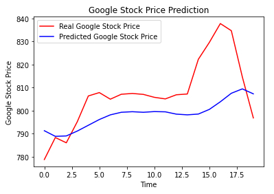
Finally, the predicted and actual values are displayed:
# Visualising the results
plt.plot(real_stock_price, color = 'red', label = 'Real Google Stock Price')
plt.plot(predicted_stock_price, color = 'blue', label = 'Predicted Google Stock Price')
plt.title('Google Stock Price Prediction')
plt.xlabel('Time')
plt.ylabel('Google Stock Price')
plt.legend()
plt.show()\

ID:(13884, 0)
