
Mixing processes in shallow waters
Storyboard 
Mixing mechanisms in shallow areas are generated by various types of waves. Among them are internal waves, surface waves, wave-current interaction, tides, and wave breaking on the coast.
ID:(1629, 0)
Shallow mixing mechanisms
Image
Para el caso en el borde costero en donde hay baja profundidad se tienen los siguientes mecanismos que contribuyen el mezclado de las aguas por efecto de:
• olas internas
adicionalmente existen contribuciones adicionales mediante
• mezcla por ola
• interacción de corriente con olas
• mezcla por mares
• mezcla por quiebre de olas en costa
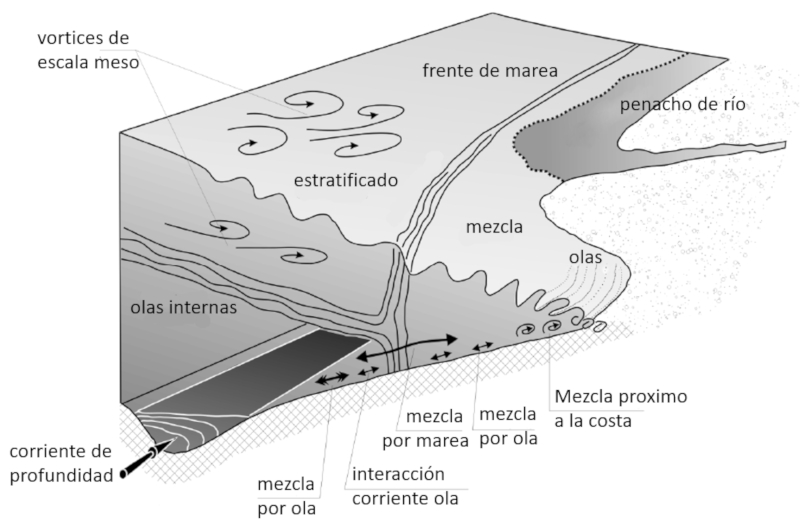
De Coastal Ocean Turbulence and Mixing, A.J. Souza, H. Burchard, C. Eden, C. Pattiaratchi, and H. van Haren, Coupled Coastal Wind, Wave and Current Dynamics (eds C. Mooers, P.Craig, N. Huang), Cambridge University Press (Cambridge, UK).
ID:(12196, 0)
Disturbance magnitudes
Image
Las perturbaciones se pueden ordenar en función de sus escalas de tiempo y dimensiones. El resultado se presenta en la siguiente grafica:
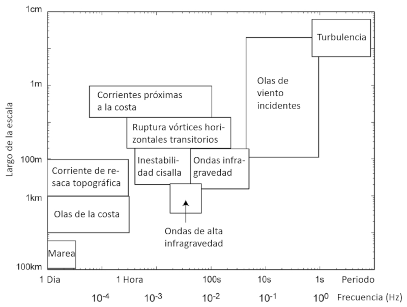
De Coastal Ocean Turbulence and Mixing, A.J. Souza, H. Burchard, C. Eden, C. Pattiaratchi, and H. van Haren, Coupled Coastal Wind, Wave and Current Dynamics (eds C. Mooers, P.Craig, N. Huang), Cambridge University Press (Cambridge, UK).
ID:(12200, 0)
Strouhal number as a function of Reynold number
Image
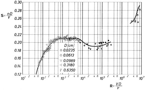
The strouhal number ($St$) is empirically related to the reynolds number ($Re$). The strouhal number ($St$) is associated with the vortex generation frequency ($\omega$), the friction speed ($U_d$), and the total depth ($H$) is
| $ St \equiv \displaystyle\frac{ \omega H }{ U_d }$ |
This allows estimating, via the reynolds number ($Re$), the frequency at which concentration can exchange the components to be diffused. However, it must be kept in mind that the process may be aborted if the frequency is lower than that of the tides.
ID:(12199, 0)
Kinematic stress
Description
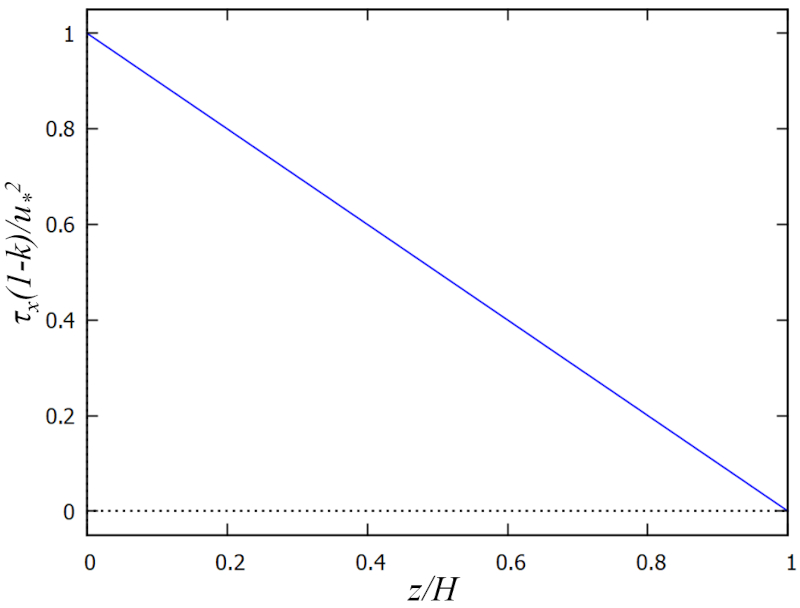
If it is assumed that there is no wind on the surface, it can be assumed that there is no tension on it. Therefore, there will only be water tension at the bottom. This tension will decrease linearly from the bottom to the surface. To simplify the modeling, the proportion between the depth ($z$) and the total depth ($H$) can be used, giving us a dimensionless factor the relative depth ($\xi$). The kinematic stress ($\tau_x$) will, therefore, be proportional to
$\tau_x \propto 1-\xi$
Since the kinematic stress ($\tau_x$) is equivalent to the energy density divided by the density, the value at the bottom must be proportional to the square of the velocity at the bottom. This is described in the model with the friction speed ($U_d$) and means that
$\tau_x \propto U_d^2$
Finally, there is the effect of the rugosity ($k$) of the seabed, i.e., the proportion of the unevenness ($d$) and the total depth ($H$). This means that the kinematic stress ($\tau_x$) must be corrected by a factor analogous to depth:
$\tau_x \propto \displaystyle\frac{1-\xi}{1-k}$
Thus, a model of the form is obtained:
| $ \tau_x \equiv \displaystyle\frac{ U_d ^2}{1- k }(1- \xi )$ |
which is graphed as follows:
ID:(15630, 0)
Mixing length
Description
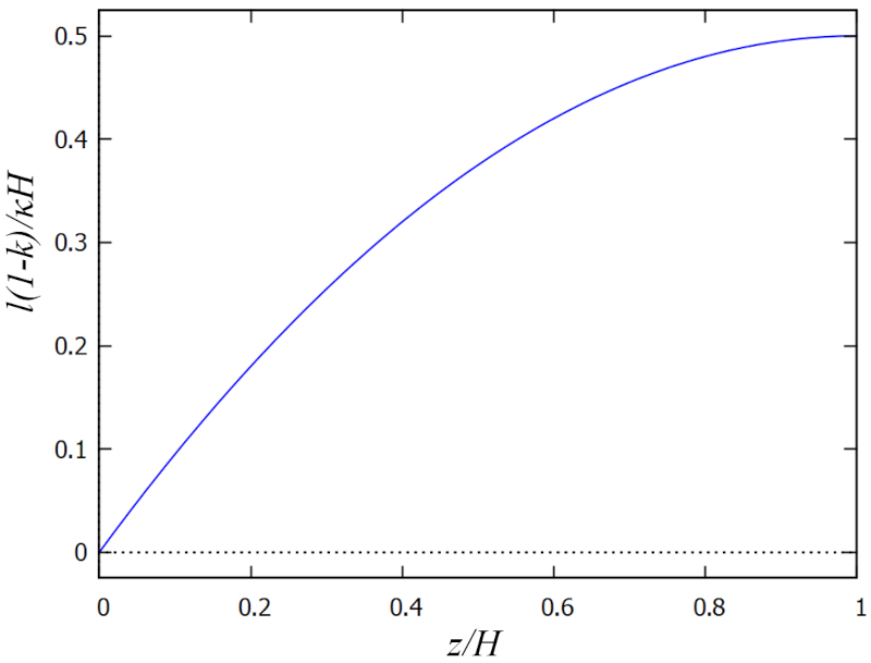
The mixing length ($l$) corresponds to what could be described as the size of the vortices. Near the wall, these can only be as large as the distance to the wall, which is minimal. As we approach the surface, they can become increasingly larger, so the function should reach a maximum at this point.
To simplify the modeling, the proportion between the depth ($z$) and the total depth ($H$) can be used, giving us a dimensionless factor the relative depth ($\xi$). Thus, a simple function that meets this description is:
$l \propto \xi\left(1-\displaystyle\frac{1}{2}\xi\right)$
On the other hand, Prandtl's boundary layer model shows that these are a fraction of the flow with a width equal to the total depth ($H$) and a proportion of the karman constant ($\kappa$), so:
$l \propto \kappa H$
Finally, we must correct for the effect of roughness in the same way as for the kinematic stress:
$l \propto \displaystyle\frac{\kappa H}{1-k}$
Therefore, the mixing length ($l$) can be modeled as follows:
| $ l \equiv \displaystyle\frac{ \kappa H }{1 - k } \xi \left(1 - \displaystyle\frac{1}{2} \xi \right)$ |
ID:(12201, 0)
Eddy viscosity
Concept
When Prandtl models the formation of eddies near walls, he establishes the relationship between the eddy viscosity ($A$), the mixing length ($l$), and the gradient of the velocity profile ($u_z$) in the depth ($z$) as follows:
| $ A = l ^2\displaystyle\frac{\partial u_z }{\partial z }$ |
On the other hand, the typical viscous force, which is modeled as viscosity multiplied by the contact surface and the velocity gradient, corresponds to the kinematic stress ($\tau_x$) in the case of turbulence:
| $ \tau_x = A \displaystyle\frac{\partial u_z }{\partial z }$ |
From both equations, the relationship emerges:
| $ \tau_x = \displaystyle\frac{ A ^2 }{ l ^2 }$ |
This relationship allows calculating the eddy viscosity ($A$) as a function of the kinematic stress ($\tau_x$) and the mixing length ($l$), which are modeled in this case. Thus, with the total depth ($H$), the friction speed ($U_d$), the rugosity ($k$), the relative depth ($\xi$), and the karman constant ($\kappa$):
| $ A = \displaystyle\frac{ \kappa H U_d }{(1- k )^{3/2}} \xi \left(1- \displaystyle\frac{1}{2} \xi \right)\sqrt{1- \xi }$ |
which is represented below:
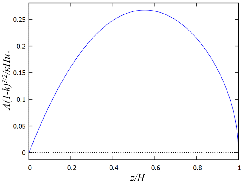
The result is that turbulent viscosity is maximal at mid-depth and reduces to minimal values both near the bottom and near the surface. In other words, in these zones, mixing and momentum loss are lower.
ID:(15624, 0)
Velocity profile
Concept
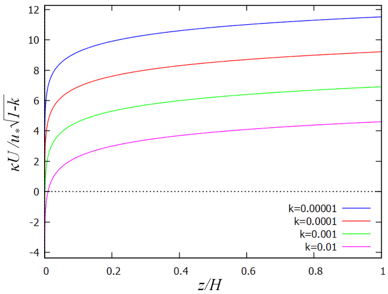
Since the kinematic stress ($\tau_x$) is equal to the eddy viscosity ($A$) and the gradient of the velocity profile ($u_z$) in the depth ($z$), the equation can be integrated to obtain the velocity profile:
$u_z = \displaystyle\int_d^z \frac{\tau_x}{A} , dz'$
After integrating this expression, with the friction speed ($U_d$), the karman constant ($\kappa$), the rugosity ($k$), and the relative depth ($\xi$), we obtain:
| $ u_z = \displaystyle\frac{ U_d }{ \kappa }\sqrt{1-k}\ln\left(\displaystyle\frac{ \xi }{ k }\right)$ |
which corresponds to the famous logarithmic law developed by Prandtl and Schlichting.
The profile is shown in the following graph:
The profile also allows relating the velocidad en la superficie ($U$) with the friction speed ($U_d$) as a function of the rugosity ($k$) and the karman constant ($\kappa$), which in turn allows defining a ERROR:9468 with:
| $ U ^2 = \displaystyle\frac{ U_d ^2}{ C_D }$ |
and
| $ C_D = \displaystyle\frac{ \kappa ^2 }{(1- k ) \ln^2(1/ k )}$ |
ID:(15623, 0)
Sediment concentration
Concept
If we consider the behavior of suspended material, we'll observe two main factors. Firstly, there's a tendency for it to sediment with a velocity the sedimentation rate ($\omega_s$), generating a flow dependent on the concentración de sedimentos ($c_z$), expressed as:
$\omega_s c_z$
On the other hand, eddies tend to mix the water, generating a diffusion that carries sediments towards the surface. This flow, represented by the eddy viscosity ($A$), is given by the gradient of the concentración de sedimentos ($c_z$) in the depth ($z$), equal to:
$A\displaystyle\frac{\partial c_z}{\partial z}$
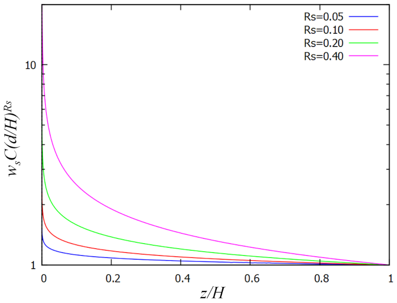
The distribution forms when sediments reach equilibrium, where the sedimentation flow equals the diffusion generated by eddies towards the surface. Integrating both terms of the equation with the erosion rate ($E$) and the unevenness ($d$), we obtain the distribution:
$c_z=\displaystyle\frac{E}{\omega_s}e^{\displaystyle\int_d^z \omega_s/A dz'}$
After employing the expression obtained for the eddy viscosity ($A$) with the rouse factor ($R_s$), the rugosity ($k$), and the relative depth ($\xi$), we derive the expression:
| $ c_z = \displaystyle\frac{ E }{ \omega_s }\left(\displaystyle\frac{ k }{ \xi }\right)^{ R_s }$ |
which can be graphically represented as:
ID:(15631, 0)
Mixing processes in shallow waters
Model
Mixing mechanisms in shallow areas are generated by various types of waves. Among them are internal waves, surface waves, wave-current interaction, tides, and wave breaking on the coast.
Variables
Calculations
Calculations
Equations
None
(ID 12182)
Just as the kinematic stress ($\tau_x$) relates to the eddy viscosity ($A$) and the mixing length ($l$), it follows that:
| $ \tau_x = \displaystyle\frac{ A ^2 }{ l ^2 }$ |
If the karman constant ($\kappa$), the total depth ($H$), and the rugosity ($k$) are used:
| $ l \equiv \displaystyle\frac{ \kappa H }{1 - k } \xi \left(1 - \displaystyle\frac{1}{2} \xi \right)$ |
and with the friction speed ($U_d$):
| $ \tau_x \equiv \displaystyle\frac{ U_d ^2}{1- k }(1- \xi )$ |
we obtain:
| $ A = \displaystyle\frac{ \kappa H U_d }{(1- k )^{3/2}} \xi \left(1- \displaystyle\frac{1}{2} \xi \right)\sqrt{1- \xi }$ |
(ID 12185)
Just as the kinematic stress ($\tau_x$) relates to the eddy viscosity ($A$), the velocity profile ($u_z$), and the depth ($z$), it is defined by
| $ \tau_x = A \displaystyle\frac{\partial u_z }{\partial z }$ |
and can be integrated from the unevenness ($d$) to the depth ($z$) to obtain the velocity using the following expression:
$u_z=\displaystyle\int_d^z\displaystyle\frac{\tau_x}{A}dz'$
With the formulation of the eddy viscosity ($A$) in terms of the relative depth ($\xi$) along with the total depth ($H$), the rugosity ($k$), and the friction speed ($U_d$), and considering that
the following equation for velocity is derived:
$u_z=\displaystyle\frac{U_d\sqrt{1-k}}{\kappa}(\ln(z/d) + \Phi(\xi,k))$
where
$\Phi=2[\arctan(\lambda)-\arctan(\lambda_0)]-\ln\left(\displaystyle\frac{1+\lambda}{1+\lambda_0}\right)$
is defined with
$\lambda=\sqrt{1-\xi}$
and
$\lambda=\sqrt{1-k}$
Since throughout much of the depth
$\ln(z/d) \gg \Phi(\xi,k)$
the velocity profile can be simplified to
| $ u_z = \displaystyle\frac{ U_d }{ \kappa }\sqrt{1-k}\ln\left(\displaystyle\frac{ \xi }{ k }\right)$ |
(ID 12187)
Sediments tend to settle to the bottom with a sedimentation rate ($\omega_s$), while diffusion, which in this case corresponds to the mixing generated by eddies, induces a flow equal to the eddy viscosity ($A$) and the gradient of the concentración de sedimentos ($c_z$) in the depth ($z$) as follows:
$A\displaystyle\frac{\partial c_z}{\partial z}+\omega_s c_z= 0$
Integrating this expression gives:
$c_z = \displaystyle\frac{E}{\omega_s}e^{-\displaystyle\int_d^z \omega_s/A dz'}$
with the mixing length ($l$):
| $ \tau_x = \displaystyle\frac{ A ^2 }{ l ^2 }$ |
we have:
$c_z=\displaystyle\frac{E}{\omega_s}e^{-\displaystyle\int_d^z \omega_s/l\sqrt{\tau_x} dz'}$
which results in:
$c_z=\displaystyle\frac{E}{\omega_s}\left(\displaystyle\frac{z}{d}\right)^{R_s}\Phi_c(\xi,k)$
with the rouse factor ($R_s$) and the rouse number ($R_0$):
| $ R_s \equiv R_0 (1 - k )^{3/2}$ |
where:
$\Phi=\left(\displaystyle\frac{1+\lambda}{1+\lambda_0}\right)^{2R_s}e^{2R_s[\arctan(\lambda)-\arctan(\lambda_0)]}$
with:
$\lambda=\sqrt{1-\xi}$
and:
$\lambda=\sqrt{1-k}$
Since throughout much of the depth:
$\Phi\sim 1$
we have the concentration distribution:
| $ c_z = \displaystyle\frac{ E }{ \omega_s }\left(\displaystyle\frac{ k }{ \xi }\right)^{ R_s }$ |
(ID 12193)
Just as the eddy viscosity ($A$) is related to the mixing length ($l$), the velocity profile ($u_z$) and the depth ($z$) are defined as
| $ A = l ^2\displaystyle\frac{\partial u_z }{\partial z }$ |
and since the kinematic stress ($\tau_x$) is
| $ \tau_x = A \displaystyle\frac{\partial u_z }{\partial z }$ |
eliminating the gradient yields
| $ \tau_x = \displaystyle\frac{ A ^2 }{ l ^2 }$ |
(ID 15633)
Examples
(ID 15614)
Para el caso en el borde costero en donde hay baja profundidad se tienen los siguientes mecanismos que contribuyen el mezclado de las aguas por efecto de:
• olas internas
adicionalmente existen contribuciones adicionales mediante
• mezcla por ola
• interacci n de corriente con olas
• mezcla por mares
• mezcla por quiebre de olas en costa
De Coastal Ocean Turbulence and Mixing, A.J. Souza, H. Burchard, C. Eden, C. Pattiaratchi, and H. van Haren, Coupled Coastal Wind, Wave and Current Dynamics (eds C. Mooers, P.Craig, N. Huang), Cambridge University Press (Cambridge, UK).
(ID 12196)
Las perturbaciones se pueden ordenar en funci n de sus escalas de tiempo y dimensiones. El resultado se presenta en la siguiente grafica:
De Coastal Ocean Turbulence and Mixing, A.J. Souza, H. Burchard, C. Eden, C. Pattiaratchi, and H. van Haren, Coupled Coastal Wind, Wave and Current Dynamics (eds C. Mooers, P.Craig, N. Huang), Cambridge University Press (Cambridge, UK).
(ID 12200)
The strouhal number ($St$) is empirically related to the reynolds number ($Re$). The strouhal number ($St$) is associated with the vortex generation frequency ($\omega$), the friction speed ($U_d$), and the total depth ($H$) is
| $ St \equiv \displaystyle\frac{ \omega H }{ U_d }$ |
This allows estimating, via the reynolds number ($Re$), the frequency at which concentration can exchange the components to be diffused. However, it must be kept in mind that the process may be aborted if the frequency is lower than that of the tides.
(ID 12199)
If it is assumed that there is no wind on the surface, it can be assumed that there is no tension on it. Therefore, there will only be water tension at the bottom. This tension will decrease linearly from the bottom to the surface. To simplify the modeling, the proportion between the depth ($z$) and the total depth ($H$) can be used, giving us a dimensionless factor the relative depth ($\xi$). The kinematic stress ($\tau_x$) will, therefore, be proportional to
$\tau_x \propto 1-\xi$
Since the kinematic stress ($\tau_x$) is equivalent to the energy density divided by the density, the value at the bottom must be proportional to the square of the velocity at the bottom. This is described in the model with the friction speed ($U_d$) and means that
$\tau_x \propto U_d^2$
Finally, there is the effect of the rugosity ($k$) of the seabed, i.e., the proportion of the unevenness ($d$) and the total depth ($H$). This means that the kinematic stress ($\tau_x$) must be corrected by a factor analogous to depth:
$\tau_x \propto \displaystyle\frac{1-\xi}{1-k}$
Thus, a model of the form is obtained:
| $ \tau_x \equiv \displaystyle\frac{ U_d ^2}{1- k }(1- \xi )$ |
which is graphed as follows:
(ID 15630)
The mixing length ($l$) corresponds to what could be described as the size of the vortices. Near the wall, these can only be as large as the distance to the wall, which is minimal. As we approach the surface, they can become increasingly larger, so the function should reach a maximum at this point.
To simplify the modeling, the proportion between the depth ($z$) and the total depth ($H$) can be used, giving us a dimensionless factor the relative depth ($\xi$). Thus, a simple function that meets this description is:
$l \propto \xi\left(1-\displaystyle\frac{1}{2}\xi\right)$
On the other hand, Prandtl's boundary layer model shows that these are a fraction of the flow with a width equal to the total depth ($H$) and a proportion of the karman constant ($\kappa$), so:
$l \propto \kappa H$
Finally, we must correct for the effect of roughness in the same way as for the kinematic stress:
$l \propto \displaystyle\frac{\kappa H}{1-k}$
Therefore, the mixing length ($l$) can be modeled as follows:
| $ l \equiv \displaystyle\frac{ \kappa H }{1 - k } \xi \left(1 - \displaystyle\frac{1}{2} \xi \right)$ |
(ID 12201)
When Prandtl models the formation of eddies near walls, he establishes the relationship between the eddy viscosity ($A$), the mixing length ($l$), and the gradient of the velocity profile ($u_z$) in the depth ($z$) as follows:
| $ A = l ^2\displaystyle\frac{\partial u_z }{\partial z }$ |
On the other hand, the typical viscous force, which is modeled as viscosity multiplied by the contact surface and the velocity gradient, corresponds to the kinematic stress ($\tau_x$) in the case of turbulence:
| $ \tau_x = A \displaystyle\frac{\partial u_z }{\partial z }$ |
From both equations, the relationship emerges:
| $ \tau_x = \displaystyle\frac{ A ^2 }{ l ^2 }$ |
This relationship allows calculating the eddy viscosity ($A$) as a function of the kinematic stress ($\tau_x$) and the mixing length ($l$), which are modeled in this case. Thus, with the total depth ($H$), the friction speed ($U_d$), the rugosity ($k$), the relative depth ($\xi$), and the karman constant ($\kappa$):
| $ A = \displaystyle\frac{ \kappa H U_d }{(1- k )^{3/2}} \xi \left(1- \displaystyle\frac{1}{2} \xi \right)\sqrt{1- \xi }$ |
which is represented below:
The result is that turbulent viscosity is maximal at mid-depth and reduces to minimal values both near the bottom and near the surface. In other words, in these zones, mixing and momentum loss are lower.
(ID 15624)
Since the kinematic stress ($\tau_x$) is equal to the eddy viscosity ($A$) and to the gradient of the velocity profile ($u_z$) with respect to the depth ($z$), the equation can be integrated to obtain the velocity profile:
$u_z = \displaystyle\int_d^z \frac{\tau_x}{A} dz'$
After performing the integration, and using the friction speed ($U_d$), the karman constant ($\kappa$), the rugosity ($k$), and the relative depth ($\xi$), we obtain:
| $ u_z = \displaystyle\frac{ U_d }{ \kappa }\sqrt{1-k}\ln\left(\displaystyle\frac{ \xi }{ k }\right)$ |
This expression corresponds to the well-known logarithmic law of velocity profiles developed by Prandtl and Schlichting.
The result is shown in the following graph:
The profile also allows a relationship to be established between the velocidad en la superficie ($U$) and the friction speed ($U_d$) as a function of the drag coefficient ($C_D$):
| $ U ^2 = \displaystyle\frac{ U_d ^2}{ C_D }$ |
In turn, the drag coefficient ($C_D$) can be estimated from the rugosity ($k$) and the karman constant ($\kappa$) using:
| $ C_D = \displaystyle\frac{ \kappa ^2 }{(1- k ) \ln^2(1/ k )}$ |
(ID 15623)
If we consider the behavior of suspended material, we'll observe two main factors. Firstly, there's a tendency for it to sediment with a velocity the sedimentation rate ($\omega_s$), generating a flow dependent on the concentración de sedimentos ($c_z$), expressed as:
$\omega_s c_z$
On the other hand, eddies tend to mix the water, generating a diffusion that carries sediments towards the surface. This flow, represented by the eddy viscosity ($A$), is given by the gradient of the concentración de sedimentos ($c_z$) in the depth ($z$), equal to:
$A\displaystyle\frac{\partial c_z}{\partial z}$
The distribution forms when sediments reach equilibrium, where the sedimentation flow equals the diffusion generated by eddies towards the surface. Integrating both terms of the equation with the erosion rate ($E$) and the unevenness ($d$), we obtain the distribution:
$c_z=\displaystyle\frac{E}{\omega_s}e^{\displaystyle\int_d^z \omega_s/A dz'}$
After employing the expression obtained for the eddy viscosity ($A$) with the rouse factor ($R_s$), the rugosity ($k$), and the relative depth ($\xi$), we derive the expression:
| $ c_z = \displaystyle\frac{ E }{ \omega_s }\left(\displaystyle\frac{ k }{ \xi }\right)^{ R_s }$ |
which can be graphically represented as:
(ID 15631)
(ID 15618)
ID:(1629, 0)