Concept of a sequential model for images
Image 
In the case of structuring a model to process images, the information of the images must be condensed (high number of pixels) to recognize a limited number of categories. For this, two types of actions are used:
- convolution (Conv2D)
- averaging (Pooling)
After one or more convolutions and averages, the points are tied to an arrangement that is associated with the forecast to be made:

Conv2D(filters=32, kernel_size=(3,3), activation='relu', padding='same',input_shape=(224,224,3)),
MaxPool2D(pool_size=(2,2), strides=2),
Conv2D(filters=64, kernel_size=(3,3), activation='relu', padding='same'),
MaxPool2D(pool_size=(2,2), strides=2),
Flatten(),
Dense(units=len(classes),activation='softmax'),
ID:(13784, 0)
Meaning of convolution
Image 
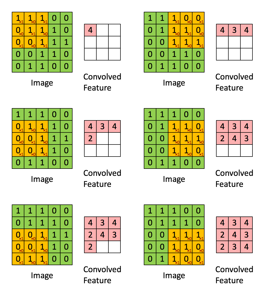
The convolution operation is analogous to multiplication by a matrix that corresponds to a rotation of a vector. In this sense, convolutions can be understood as a parameterization of a rotation of the image to be adjusted in the learning process:
ID:(13785, 0)
Calculation of the convolution
Image 
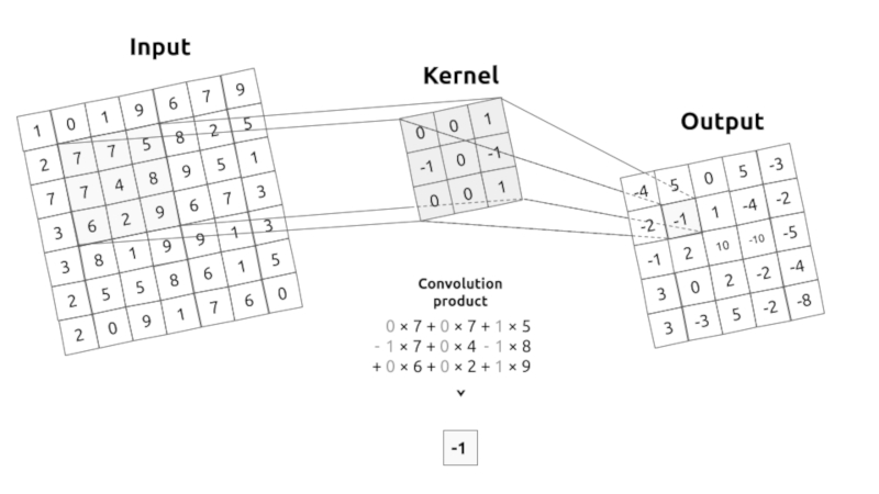
The convolution corresponds to the multiplication of elements of a section of the image by a kernel matrix whose sum is taken as the result of the convolution:
Conv2D(filters=32, kernel_size=(3,3), activation='relu', padding='same',input_shape=(224,224,3)),
ID:(13786, 0)
Summarize calculation (pooling)
Image 
Image sections are summarized by the pooling process, one of this type of process being to obtain the maximum value (MaxPooling)
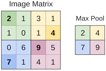
MaxPool2D(pool_size=(2,2), strides=2)
ID:(13787, 0)
Another type of summarize calculation (pooling)
Image 
A different method of summarization is to obtain an average value for a section of the image (AvgPooling)
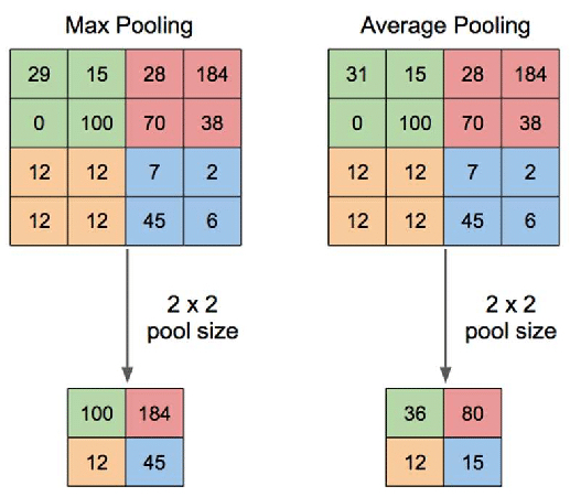
ID:(13788, 0)
Value filter (activation)
Image 
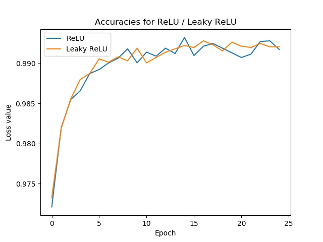
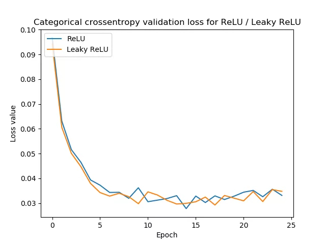
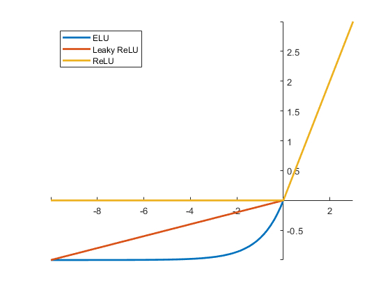
After performing the convolution, the values can be filtered according to enabling or disabling the pixels that represent the operation. For this, activation functions are used, such as those of
- ELU
- RELU
- WeakRELU
Conv2D(filters=32, kernel_size=(3,3), activation='relu', padding='same',input_shape=(224,224,3)),
ID:(13789, 0)
Image sequential model
Description 
The basic sequential model that can be defined must have:
- a convolution process on the initial images
- a maxpooling process to reduce the number of points
- a second convolution process on the already reduced image
- a second maxpooling process to reduce the number of points again
- the transition to a line array (flatten)
- an association to the desired result represented by a dense array (completely connected to previous line array)
import numpy as np
import tensorflow as tf
from tensorflow import keras
from tensorflow.keras.models import Sequential
from tensorflow.keras.layers import Activation, Dense, Flatten, BatchNormalization, Conv2D, MaxPool2D
from tensorflow.keras.optimizers import Adam
from tensorflow.keras.metrics import categorical_crossentropy
from tensorflow.keras.preprocessing.image import ImageDataGenerator
from sklearn.metrics import confusion_matrix

# basic image sequential model: 2 convolutions, 2 maxpoolings, a flatten layer and a final dense layer
base_model = Sequential([
    Conv2D(filters=32, kernel_size=(3,3), activation='relu', padding='same',input_shape=(224,224,3)),
    MaxPool2D(pool_size=(2,2), strides=2),
    Conv2D(filters=64, kernel_size=(3,3), activation='relu', padding='same'),
    MaxPool2D(pool_size=(2,2), strides=2),
    Flatten(),
    Dense(units=len(classes),activation='softmax'),
])
It is important to take care that
The size of the images prepared with the ImageDataGenerator command must match that defined under input_shape. In this case it is 224 x 224 and the three values of the colors (RGB).
The number of units in the final plane (dense layer) must coincide with the number of classes that are being defined.
ID:(13755, 0)
Show model structure
Description 
base_model.summary()
Model: 'sequential'
_________________________________________________________________
Layer (type) Output Shape Param #
=================================================================
conv2d_2 (Conv2D) (None, 224, 224, 32) 896
_________________________________________________________________
max_pooling2d_2 (MaxPooling2 (None, 112, 112, 32) 0
_________________________________________________________________
conv2d_3 (Conv2D) (None, 112, 112, 64) 18496
_________________________________________________________________
max_pooling2d_3 (MaxPooling2 (None, 56, 56, 64) 0
_________________________________________________________________
flatten_1 (Flatten) (None, 200704) 0
_________________________________________________________________
dense_7 (Dense) (None, 25) 5017625
=================================================================
Total params: 5,037,017
Trainable params: 5,037,017
Non-trainable params: 0
_________________________________________________________________
ID:(13756, 0)
Build model
Description 
To carry out the learning, it is first necessary to configure (compile) the model, which is done with the command:
base_model.compile(optimizer=Adam(learning_rate=0.0001), loss='categorical_crossentropy',metrics=['accuracy'])
ID:(13757, 0)
Learning process
Description 
The model is trained with the fit function in which it is indicated the data to train under x (in this case train_batches), the data to validate under validation_data< /b> (in this case valid_batches) in a number of stages called epochs showing the results verbose.# learn with the train_batches and validate with the validate_batches
base_model.fit(x=train_batches, validation_data=validate_batches, epochs=10,verbose=2)
Epoch 1/10
373/373 - 78s - loss: 16.3827 - accuracy: 0.2999 - val_loss: 2.1490 - val_accuracy: 0.3582
Epoch 2/10
373/373 - 78s - loss: 0.6922 - accuracy: 0.7854 - val_loss: 2.3907 - val_accuracy: 0.4011
Epoch 3/10
373/373 - 77s - loss: 0.1305 - accuracy: 0.9734 - val_loss: 2.5407 - val_accuracy: 0.4040
Epoch 4/10
373/373 - 77s - loss: 0.0335 - accuracy: 0.9944 - val_loss: 3.0110 - val_accuracy: 0.4140
Epoch 5/10
373/373 - 77s - loss: 0.0118 - accuracy: 0.9987 - val_loss: 3.3895 - val_accuracy: 0.4011
Epoch 6/10
373/373 - 77s - loss: 0.0088 - accuracy: 0.9989 - val_loss: 3.0567 - val_accuracy: 0.4327
Epoch 7/10
373/373 - 76s - loss: 0.0023 - accuracy: 1.0000 - val_loss: 3.2413 - val_accuracy: 0.4341
Epoch 8/10
373/373 - 76s - loss: 0.0012 - accuracy: 1.0000 - val_loss: 3.4144 - val_accuracy: 0.4312
Epoch 9/10
373/373 - 77s - loss: 7.5812e-04 - accuracy: 1.0000 - val_loss: 3.4770 - val_accuracy: 0.4312
Epoch 10/10
373/373 - 77s - loss: 5.3013e-04 - accuracy: 1.0000 - val_loss: 3.5489 - val_accuracy: 0.4355
It is important to avoid overfitting, so it is often necessary to work with a not very large number of stages.
ID:(13758, 0)
Store models
Image 
To store a model, execute the save command:
# almacenar modelos
directory = 'F:/go/face_scrapper/faces/base_model_20210721'
base_model.save('F:/go/face_scrapper/faces/base_model_20210721')
INFO:tensorflow:Assets written to: F:/go/face_scrapper/faces/base_model_20210721\assets
with which a folder is generated with the name of the directory, the model file and the variables and assets folders:

ID:(13797, 0)
Load models
Description 
To store a model, execute the save command:
# load models
directory = 'F:/go/face_scrapper/faces/base_model_20210721'
new_model = tf.keras.models.load_model(directory)
ID:(13798, 0)

