Deep circulation flows
Storyboard 
There are several points where flows from the ocean surface to greater depths occur, inducing deep circulation. This circulation is subject to the Coriolis force, resulting in deviations and some flows towards the surface (upwelling) that are associated with surface currents.
The classic model for these currents is that of Stommel and Arons, which, although simple, explains the different depth flows observed.
[1] Ocean Circulation Theory, Joseph Pedlosky, Springer 1998 (7.3 Stommel-Arons Theory: Abyssal Flow on the Sphere)
ID:(1623, 0)
Thermohaline circulation
Concept 
The deeper circulation is known as thermohaline circulation (THC) because its movement is associated with variations in temperature (thermo) and salinity (haline). To understand how this occurs, we must first describe the structure of the system.
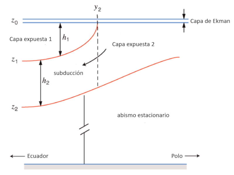
In a simplified form, the ocean can be modeled as a three-layer system:
- An upper layer where water movement is generated by wind-driven currents.
- An intermediate layer where movement is driven by density differences in the ocean, originating from variations in temperature and salinity (thermohaline).
- A deep layer that can be assumed to be at rest.
The increase in density towards the poles, where the water is colder, causes the water to literally sink, creating subduction beneath the surface layer. The following diagram summarizes the described process:
ID:(12095, 0)
Thermohaline circulation over the planet
Description 
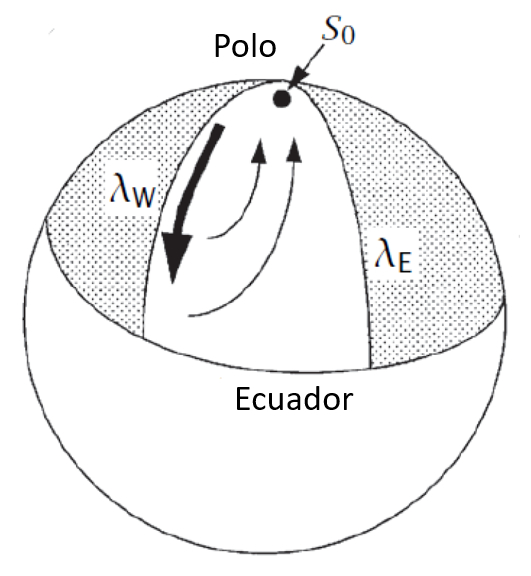
If we observe the globe, the thermohaline circulation is generated near one of the poles (north or south) through water that, due to higher salinity and lower temperature, begins to sink. Its flow is directed towards the equator, creating an upwelling where water partially rises and flows towards the pole to replenish the descending water.
Representation of the North Atlantic in the Stommel and Arons model [1], [2]
[1] Stommel, H., & Arons, A. B. (1960). On the abyssal circulation of the world oceanI. Stationary planetary flow patterns on a sphere. Deep Sea Research (1953), 6(2), 140-154.
[2] Stommel, H., & Arons, A. B. (1960). On the abyssal circulation of the world oceanII. An idealized model of the circulation pattern and amplitude in oceanic basins. Deep Sea Research (1953), 6(3), 217-233.
ID:(12096, 0)
Box model
Description 
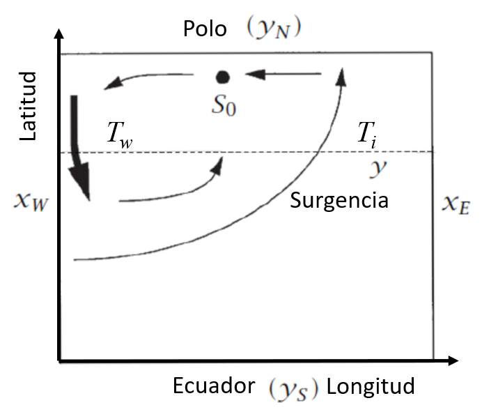
The Stommel and Arons model [1], [2] considers the ocean as a two-dimensional box with coordinates on the x and y axes. Specifically:
- Coordinates on the x-axis: $x_w$ (west) and $x_e$ (east).
- Coordinates on the y-axis: $y_s$ (south) and $y_n$ (north).
These coordinates are represented in the following graph:
Atlantic box model [1], [2].
[1] Stommel, H., & Arons, A. B. (1960). On the abyssal circulation of the world oceanI. Stationary planetary flow patterns on a sphere. Deep Sea Research (1953), 6(2), 140-154.
[2] Stommel, H., & Arons, A. B. (1960). On the abyssal circulation of the world oceanII. An idealized model of the circulation pattern and amplitude in oceanic basins. Deep Sea Research (1953), 6(3), 217-233.
ID:(12082, 0)
Characteristic times
Description 
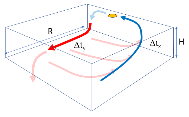
Each stage is associated with a characteristic time:
- Travel time with the main flow $\Delta t_y$
- Deflection time with the loss flow $\Delta t_x$
- Upwelling time $\Delta t_z$
ID:(13426, 0)
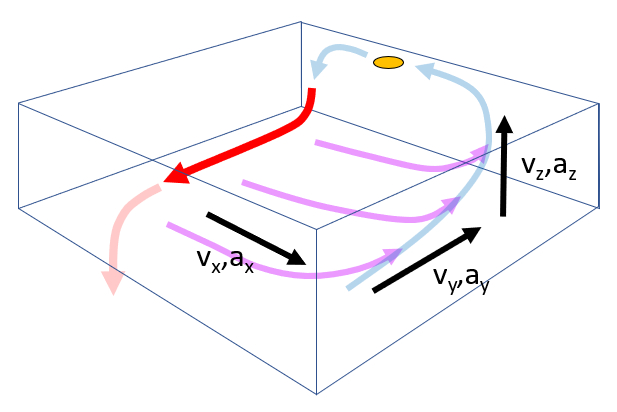
Velocities and Accelerations per Flow
Description 
Each characteristic time is associated with velocities and accelerations along the traveled path:
- With the main flow $v_y, a_y$.
- With the loss flow $v_x, a_x$.
- With the upwelling $v_z, a_z$.
Generally, the initial velocity (
ID:(13427, 0)
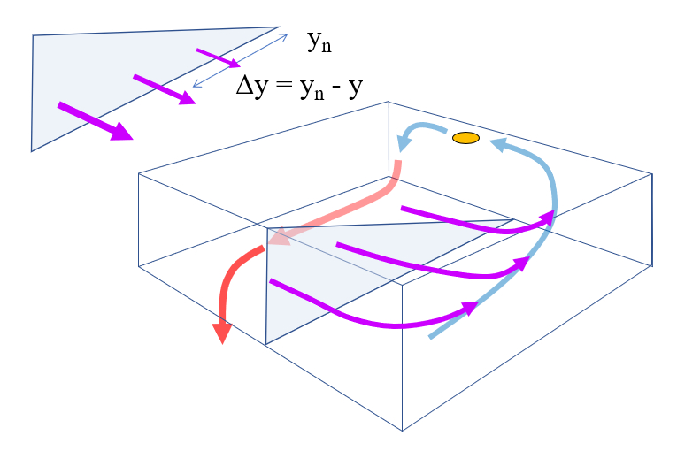
Lost Flow Geometry
Description 
The loss flow is not uniform and is distributed along the latitude, so it is modeled based on its distance from the northernmost position. Thus, it is zero at northern latitudes and maximum at the southern edge of the rectangle where the circulation is modeled:
ID:(13428, 0)
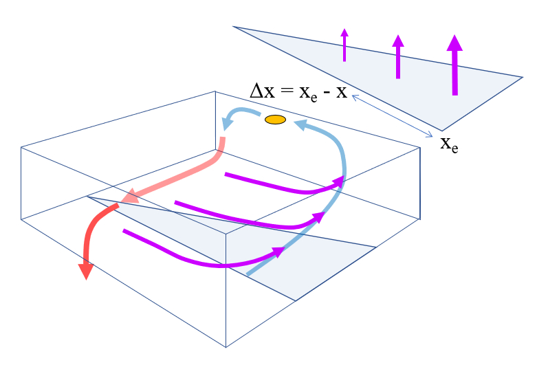
Upwelling flow geometry
Description 
Since the loss flow is not uniform, neither is the upwelling. Within the same model, it is assumed that the upwelling is maximum at the eastern edge of the rectangle where the circulation is modeled. Similar to the loss, a linear relationship is assumed:
ID:(13429, 0)
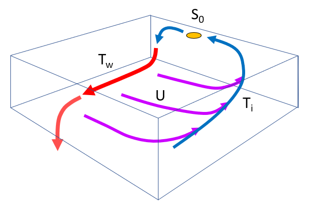
Main flows of deep currents
Description 
There are four flows to consider in modeling deep flow:
The main flow $F_w$, which moves along the seafloor.
The loss flow $F_i$, which is the fraction deviated due to the Coriolis force.
The upwelling flow $U_x$, which corresponds to the fraction of loss flow reaching the surface.
The sinking flow $S_0, originating from surface currents, including losses that sink again.
ID:(13425, 0)
Underwater currents and Coriolis
Description 
The so-called Coriolis force plays an essential role in the dynamics of water in the poles, influencing how water masses descend due to variations in temperature and salinity.
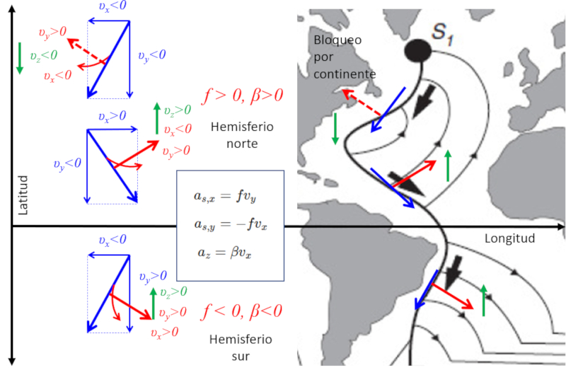
When analyzing the Atlantic Ocean, one can observe a movement of water from the pole towards the equator, which deflects towards the west. This phenomenon is caused by the lag relative to the planet\'s rotation, as it transitions from a zone of slower speed along the latitude to one of higher speed. This behavior can be modeled using the Coriolis equation for the x-direction, given by :
| $ a_{s,x} = f v_y $ |
In this equation, the Coriolis factor
The geographical contour of the continent allows for movement in the x-direction (longitude), resulting in an acceleration in the y-direction (latitude), which can be calculated using :
| $ a_{s,y} = - f v_x $ |
This calculation reveals that near the equator, displacements occur that take water away from the main current, moving it northward. If we examine the acceleration in the z-direction (depth) and take into account that
| $ a_{cz} = R \beta v_x $ |
.
ID:(12122, 0)
Stommel-Arons depth flows
Description 
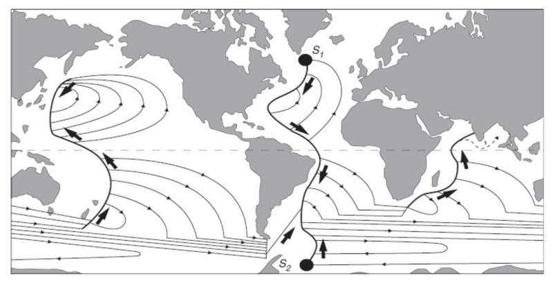
At the end, Stommel and Arons [1], [2] solve the model, indicating the main deep flows that exist throughout the globe:
[1] Stommel, H., & Arons, A. B. (1960). On the abyssal circulation of the world oceanI. Stationary planetary flow patterns on a sphere. Deep Sea Research (1953), 6(2), 140-154.
[2] Stommel, H., & Arons, A. B. (1960). On the abyssal circulation of the world oceanII. An idealized model of the circulation pattern and amplitude in oceanic basins. Deep Sea Research (1953), 6(3), 217-233.
ID:(12099, 0)
Structure of the Stommel-Arons model
Description 
When Stommel and Arons [1], [2] developed their first model of thermohaline circulation, they subdivided the different oceans into zones with defined upwelling (upward arrows) and two sources, one in the Arctic and the other in Antarctica:
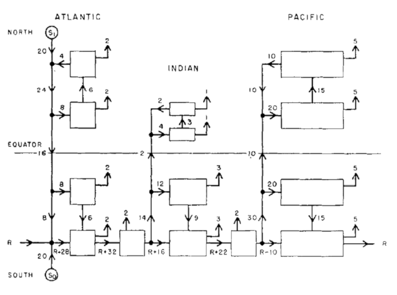
Global circulation model in Sv (Sverdrup) ($10^6 m^3/s$) [2].
[1] Stommel, H., & Arons, A. B. (1960). On the abyssal circulation of the world oceanI. Stationary planetary flow patterns on a sphere. Deep Sea Research (1953), 6(2), 140-154.
[2] Stommel, H., & Arons, A. B. (1960). On the abyssal circulation of the world oceanII. An idealized model of the circulation pattern and amplitude in oceanic basins. Deep Sea Research (1953), 6(3), 217-233.
ID:(12098, 0)
True thermohaline circulation
Description 
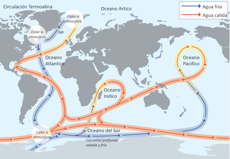
Measurements have shown that the thermohaline circulation is an integrated system that spans the entire globe. It has at least two points that can be considered as sources, and its path extends across all the oceans.
ID:(12097, 0)
Study of the possible collapse of the deep flow
Description 
Through multiple simulations, the effects of polar ice melting on the suppression of sinking and its impact on deep circulation are studied. There are indications that circulation has started to decline; however, the collapse of deep circulation does not necessarily imply the same will happen to surface circulation, which is driven by winds. What could happen is a shift in the surface circulation, resulting in a reduction of the Gulf Stream's contribution of warm waters to northern Europe.
The diagram below shows variations in flow in units of Sv (Sverdrup), which is equivalent to $10^6,m^3/s$:
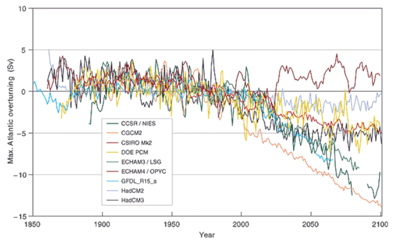
Assuming a sinking rate of approximately 20 Sv, it is concluded that in some simulations, deep circulation comes to a halt. These variations are associated with different future scenarios of human activity and considerations for aspects with less certainty about their occurrence. More detailed information can be found in the reports of the Intergovernmental Panel on Climate Change (IPCC).
ID:(13430, 0)
Model
Top 
Parameters
Variables
Calculations
Calculations
Calculations
Equations
$ a_{cz} = R \beta v_x $
a_cz = R * beta * v_x
$ \beta =\displaystyle\frac{ 2 \omega \cos \varphi }{ R }$
beta = 2* omega * cos( phi )/ R
$ f = f_0 + \beta y $
f = f_0 + beta * y
$ S_0 + T_i = T_w + U_x $
S_0 + T_i = T_w + U_x
$ S_0 = v_z \Delta x \Delta y $
S_0 = v_z * Dx * Dy
$ T_i = \displaystyle\frac{f v_z}{\beta} \Delta x $
T_i = f * v_z * Dx / beta
$ T_w =\displaystyle\frac{ S_0 }{ y_n }\left(\displaystyle\frac{ f_0 }{ \beta } + 2 y \right)$
T_w = S_0 * ( f_0 / beta + 2* y )/ y_n
$ T_w = v_z \Delta x \left(\displaystyle\frac{ f }{ \beta } + y \right) $
T_w = v_z * Dx *( f / beta + y )
$ U_x = v_z \Delta x ( y_n - y )$
U_x = v_z * Dx * ( y_n - y )
$ v_y = \displaystyle\frac{f}{\beta H} v_z $
v_y = f * v_z /( H * beta )
$ v_z =\displaystyle\frac{ \beta }{ f }\displaystyle\frac{ \Delta t_z }{ \Delta t_y } R v_y $
v_z = beta * R * v_y * Dt_z / ( Dt_y * f )
$ v_z(x) =\displaystyle\frac{2 v_z }{ H }( x_e - x )$
v_zx = 2* v_z * ( x_e - x )/ H
ID:(15585, 0)
Variation of the Coriolis factor in the arc
Equation 
In analogy to the Coriolis factor, we can study how the factor varies along the arc, leading us to obtain the coriolis Beta Factor ($\beta$) given by the latitude ($\varphi$), the planet radio ($R$), and the angular velocity of the planet ($\omega$) by:
In analogy to the coriolis factor ($f$) defined with the latitude ($\varphi$) and the angular velocity of the planet ($\omega$) as:
| $ f = 2 \omega \sin \varphi $ |
the factor varies in the arc $R\theta$, with the planet radio ($R$) and the latitude ($\varphi$) as the latitude, according to:
$\displaystyle\frac{\partial f}{\partial (R\varphi) }=\displaystyle\frac{ 2\omega\cos\varphi }{R}$
thus the coriolis Beta Factor ($\beta$) can be defined as:
| $ \beta =\displaystyle\frac{ 2 \omega \cos \varphi }{ R }$ |
ID:(12105, 0)
Upwelling based on Coriolis acceleration
Equation 
Based on the relationship between the Coriolis acceleration and the velocities in each axis, we can estimate the acceleration of upwelling that will occur in the circulation. Using the parameterization that depends on the sector size and latitude of the location, we obtain the coriolis acceleration in z direction ($a_{c,z}$) as a function of the coriolis Beta Factor ($\beta$), the planet radio ($R$), and the parallel speed ($v_x$):
When there is movement in the x-direction (east-west), it results in the coriolis acceleration in z direction ($a_{c,z}$) with the speed x of the object ($v_x$), the angular velocity of the planet ($\omega$), and the latitude ($\varphi$):
| $ a_{c,z} = 2 \omega v_x \cos \varphi$ |
This is complemented by the coriolis acceleration on the surface, in the x direction ($a_{s,x}$) (east-west), with the coriolis factor ($f$) and the speed y of the object ($v_y$):
| $ a_{s,x} = f v_y $ |
and the coriolis acceleration on the surface, in the y direction ($a_{s,y}$) (north-south) with the coriolis factor ($f$) and the speed x of the object ($v_x$), which is:
| $ a_{s,y} = - f v_x $ |
Where the coriolis factor ($f$) is defined as:
| $ f = 2 \omega \sin \varphi $ |
Therefore, we can introduce the coriolis Beta Factor ($\beta$), defined as:
| $ \beta =\displaystyle\frac{ 2 \omega \cos \varphi }{ R }$ |
With this, we obtain:
| $ a_{cz} = R \beta v_x $ |
ID:(12104, 0)
Relationship between upwelling and current
Equation 
The continuity of flow allows us to determine how velocities are related in each phase. In this way, we can estimate the upwelling speed ($v_z$) based on the coriolis Beta Factor ($\beta$), the coriolis factor ($f$), the characteristic time interval movement in $y$ ($\Delta t_y$), the characteristic time interval movement in $z$ ($\Delta t_z$), the planet radio ($R$), and the speed in meridian ($v_y$):
If we introduce typical timescales for each dimension, we can estimate the Coriolis accelerations as velocities divided by their typical timescales, that is:
$v_i =a_i \Delta t_i$
with
| $ a_{cz} = R \beta v_x $ |
Thus, we have:
$v_z=\beta R v_x\Delta t_z$
On the other hand, with the equation for the
$v_x=\displaystyle\frac{v_y}{f\Delta t_y}$
By replacing
| $ v_z =\displaystyle\frac{ \beta }{ f }\displaystyle\frac{ \Delta t_z }{ \Delta t_y } R v_y $ |
ID:(12089, 0)
Bottom speed
Equation 
As the upwelling velocity is determined by characteristic time interval movement in $y$ $s$, characteristic time interval movement in $z$ $s$, coriolis Beta Factor $rad/s m$, coriolis factor $rad/s$, planet radio $m$, speed in meridian $m/s$ and upwelling speed $m/s$,
| $ v_z =\displaystyle\frac{ \beta }{ f }\displaystyle\frac{ \Delta t_z }{ \Delta t_y } R v_y $ |
and the relationship between the times must comply with where the velocity is
| $ \displaystyle\frac{ R }{ \Delta t_y }\sim \displaystyle\frac{ H }{ \Delta t_z } $ |
the velocity at the bottom is given by as
.
ID:(12090, 0)
Upwelling
Equation 
The upwelling depends on the velocity towards the surface and the position within the box. Since it is greater towards the equator and relatively uniform across the width, it is modeled to vary only with the distance to the northern edge of the box:
$y_n - y$
Therefore, with , we have the upwelling flow:
ID:(12085, 0)
Upwelling velocity along the width
Equation 
The upwelling velocity is determined using the value average upwelling flow by latitude $m^3/s$, distance equator north edge $m$, position in latitude $m$, stommel and Arons model case width $m$ and upwelling speed $m/s$.
The flow inside the box can be modeled using the equation
| $ U_x = v_z \Delta x ( y_n - y )$ |
.
Specifically, it is observed that the upwelling velocity is higher towards the western edge, which can be represented with average upwelling flow by latitude $m^3/s$, distance equator north edge $m$, position in latitude $m$, stommel and Arons model case width $m$ and upwelling speed $m/s$ by
The presence of the factor 2 in the model accounts for taking an average considering the existing gradient.
ID:(12086, 0)
Flow conservation
Equation 
The conservation of flow implies that the flow moving along the east coast of America, denoted as $T_w$, and the upwelling components, represented by $U_x$, are initially generated by the sinking volume, indicated as $S_0$, in addition to those coming from circulation through upwelling. Therefore, we can express it as follows:
ID:(12087, 0)
Source model
Equation 
In this case, there are two types of flows: surface flow and flow towards or from the depth. By conservation, we can assume that the total flow flowing towards the depths at point S_0 should correspond to the total flow generated by the upwelling. The latter occurs over the entire surface and with vertical velocity, so:
ID:(12088, 0)
Flow through the bottom
Equation 
If the velocity is multiplied by average flow height $m$, coriolis Beta Factor $rad/s m$, coriolis factor $rad/s$, speed in meridian $m/s$ and upwelling speed $m/s$:
| $ v_y = \displaystyle\frac{f}{\beta H} v_z $ |
with the height
$T_i \sim v_y H \Delta x$
So, with average flow height $m$, coriolis Beta Factor $rad/s m$, coriolis factor $rad/s$, speed in meridian $m/s$ and upwelling speed $m/s$, the flow is:
ID:(12091, 0)
Output stream
Equation 
Unter Berücksichtigung der Bilanzgleichung mit average upwelling flow by latitude $m^3/s$, inflow $m^3/s$, loss flow $m^3/s$ and main flow $m^3/s$:
| $ S_0 + T_i = T_w + U_x $ |
und dem Beitrag der Quelle mit inflow $m^3/s$, stommel and Arons model case length $m$, stommel and Arons model case width $m$ and upwelling speed $m/s$, der lautet:
| $ S_0 = v_z \Delta x \Delta y $ |
sowie dem Hintergrundfluss mit coriolis Beta Factor $rad/s m$, coriolis factor $rad/s$, main flow $m^3/s$, stommel and Arons model case width $m$ and upwelling speed $m/s$:
| $ T_i = \displaystyle\frac{f v_z}{\beta} \Delta x $ |
und der Auftriebsströmung mit average upwelling flow by latitude $m^3/s$, distance equator north edge $m$, position in latitude $m$, stommel and Arons model case width $m$ and upwelling speed $m/s$:
| $ U_x = v_z \Delta x ( y_n - y )$ |
nehmen wir an, dass die Zone den Äquator erreicht (
ID:(12092, 0)
Development of the Coriolis factor
Equation 
Since the Coriolis factor is given by :
| $ f = 2 \omega \sin \varphi $ |
it can be related to the beta factor based on its variation around a position. This is because, in the Taylor expansion, we obtain:
$f \sim f_0 + \frac{df}{dy}y$
where the derivative is:
$\frac{df}{dy} = 2\omega\cos\theta = \beta$
Thus, with , we have:
ID:(12093, 0)
Output flow, independent of speed
Equation 
With coriolis Beta Factor $rad/s m$, coriolis factor $rad/s$, loss flow $m^3/s$, position in latitude $m$, stommel and Arons model case width $m$ and upwelling speed $m/s$, the equation
| $ T_w = v_z \Delta x \left(\displaystyle\frac{ f }{ \beta } + y \right) $ |
can be rewritten as
| $ f = f_0 + \beta y $ |
using coriolis Beta Factor $rad/s m$, coriolis factor $rad/s$, position in latitude $m$ and reference Coriolis factor $rad/s$,
ID:(12094, 0)
