Storyboard

ID:('ky', 1793)

Storyboard

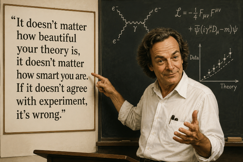
The usefulness of a scientific model depends on its ability to reproduce reality. Its parameters and the variables it calculates must be consistent with the experimental observations and with the measurements made on the system. Therefore, testing the model against the data is an essential stage of the scientific process. As Richard Feynman pointed out:

In order to carry out this validation, it is first necessary to correctly classify all the quantities involved in the model. We must distinguish between universal constants, whose values are known and do not depend on the system; external or forcing variables, which represent conditions imposed from the outside and can be modified during the simulation; structural parameters, which characterize the system and are normally determined by independent measurements; the algebraic variables, which the model calculates instantly from the state of the system and do not have temporary memory; and, finally, the dynamic or state variables, whose evolution over time constitutes the core of the model and on which its predictions are built. This classification allows us to clearly identify which information comes from the real world, which quantities are typical of the model, and which correspond to the results that can subsequently be compared with experimental observations.

ID:('gp', 654)

Storyboard

For a mathematical model to be interpreted, validated and used correctly, it is essential to classify all the quantities involved according to their origin and their temporal behavior. Not all variables play the same role: some represent information from the real world, while others are calculated by the model itself. Likewise, some remain constant during a simulation, while others evolve continuously as a consequence of the dynamics of the system. This classification determines how the model is built, how it is calibrated, and especially how it compares to experimental observations.

The figure summarizes this organization through two fundamental criteria. The first distinguishes whether a quantity is given by the user or the experiment, or if it is calculated by the model. The second distinguishes whether the quantity has temporary memory, that is, if it depends on its previous history, or if it can be calculated instantly from the current values of other variables. From the combination of both criteria, four clearly differentiated categories emerge.

1. Forcing variables (external inputs).

They correspond to external conditions that the model receives from the environment or from the experiment and that can be modified during the simulation. They are not calculated by the model and do not have their own memory. Its function is to represent the conditions under which the system operates. Typical examples are photosynthetically active radiation (PAR), air temperature, atmospheric CO concentration, relative humidity or vapor pressure deficit (VPD). In an interactive simulation they are usually the variables that the user modifies using controls or sliders.

2. Structural parameters.

They are properties of the system that remain constant during a run of the model. They describe physiological, geometric or physical characteristics of the organism and are usually obtained through independent measurements or calibration processes. Examples are maximum stomatal conductance ($g_{max}$), specific leaf area (SLA), wood density, maximum root depth or parameters of physiological curves such as BallBerry or hydraulic vulnerability coefficients. These parameters only change between simulations or during calibration processes.

3. Variables calculated algebraically (without memory).

They are quantities that the model calculates instantly using the current values of other variables. They do not store information from the past; If the inputs change, their value is completely recalculated at the same instant. Examples are stomatal conductance ($g_s$), net photosynthesis ($A_n$), transpiration rate (E) or water use efficiency (WUE), when obtained directly from the current state of the system.

4. Dynamically calculated variables (with memory).

They constitute the internal states of the model. Their evolution depends on differential equations and, therefore, they preserve memory of their history. They require an initial condition and evolve by accumulating the effects of the physical processes represented by the model. Examples include the water potential of the leaf ($\Psi_l$), the intercellular concentration of $CO_2$ ($c_i$), the water content in different compartments or the accumulated biomass. These variables represent the dynamic behavior of the system and are responsible for reproducing transient phenomena and physiological delays.

This classification not only organizes the model from a conceptual point of view, but also facilitates its computational implementation, the detection of logical errors, the calibration of parameters and validation against experimental data. In addition, it allows us to clearly identify what information comes from measurements, what properties belong to the system studied and what are truly the predictions generated by the model.

ID:('gp', 655)

Storyboard

If the equations of the model are analyzed, it will be observed that some appear formulated using derivatives or integrals with respect to time. These equations represent the dynamic part of the system, that is, those variables whose current value depends not only on the present conditions, but also on their time history.

An example is the equation:

where $\Psi_l$ corresponds to the foliar water potential and constitutes the dynamic variable with memory, since its evolution depends on the integration of flows over time. The constant $C_l$ represents the leaf water capacitance, while $F_x$ (xylem flow) and $E$ (transpiration by vapor diffusion) are dynamic variables without memory: their value can vary over time, but at each instant it is calculated directly from the current state of the system, without requiring information from previous times.

Another example is:

where $c_i$ is the concentration of $CO_2$ in the intercellular space and again constitutes a dynamic variable with memory, since its value results from integrating the balance between inputs and outputs of carbon dioxide. The constant $C_i$ represents the $CO_2$ capacitance of the intercellular space, while $A_{ns}$ (diffusive supply of $CO_2$) and $A_{nd}$ (biochemical demand for $CO_2$) are memoryless dynamic variables, whose value is determined instantaneously based on the current state of the model.

Dynamic variables with memory correspond to the states of the system. They are the only ones that preserve information from the past and, therefore, determine the temporal evolution of the model. Its calculation requires the numerical integration of the differential equations, constituting the core of the dynamic simulation described in the following sections.

ID:('gp', 692)

Storyboard

There are variables that do not appear derived or integrated with respect to time, but that can be calculated directly from dynamic variables with memory. These correspond to dynamic variables without memory, since their value changes during the simulation, although at each moment it is completely determined by the current state of the system.

An example is the xylem flow $F_x$, which is obtained from the leaf water potential $\Psi_l$, a dynamic variable with memory, together with the constants $K_h$ (effective hydraulic conductance), $L$ (hydraulic length) and the soil water potential $\Psi_s$:

In this case, $F_x$ does not require temporal integration, but evolves in time because it depends on $\Psi_l$, whose value does have memory. This dependence can be indirect, propagating through several algebraic equations. For example, the water balance is defined as:

where xylem flow $F_x$ and transpiration $E$ intervene. Both are dynamic variables without memory, since they are continuously recalculated from the state of the system, while $\Delta_b$ is simply an algebraic variable obtained as the difference between the two.

These relationships can be easily visualized in the logical network, where it is possible to follow the dependencies that arise in a dynamic variable with memory and propagate through a chain of equations until generating multiple dynamic variables without memory.



The identification of these variables is especially important because, in many real systems, dynamic variables with memory are difficult or even impossible to measure directly. On the other hand, several of the dynamic variables without memory can be observed experimentally, allowing the simulator's predictions to be compared with real measurements and validating the behavior of the model.

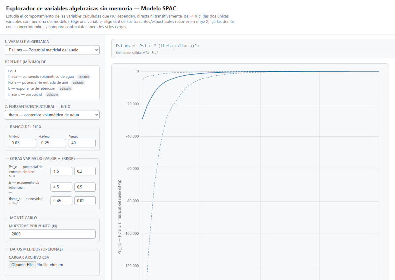
Finally, there are other algebraic variables that do not depend, either directly or indirectly, on dynamic variables with memory. These variables are not part of the temporal simulation itself, but they can be analyzed to study how they respond to changes in the forcing variables and structural variables of the model. In this way it is possible to characterize the static behavior of the system and evaluate the influence of its parameters on the calculated magnitudes.

ID:('gp', 693)

Storyboard

ID:('gp', 694)

Storyboard

ID:('gp', 696)

Storyboard

Once the model is established, it is essential to verify that it correctly describes the system we are studying. A part of the model is constituted by algebraic relations that do not vary explicitly in time. These memoryless algebraic variables depend on parameters, forcing variablessuch as temperatureand structural variables, such as the dimensions or mass of an object.

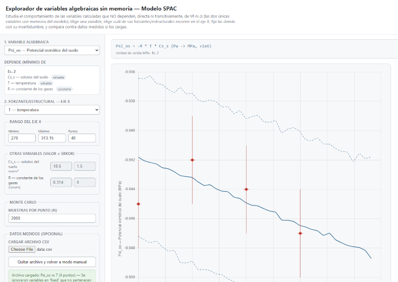
To verify that these relationships adequately represent reality, it is necessary to carry out experimental measurements of different combinations of parameters and algebraic variables, estimate the uncertainty associated with each measurement and compare the results obtained with the values predicted by the model equations.

The experimental data is stored in a file with the following format:

#algebraic=(code of the algebraic variable represented on the Y axis) #x_var=(code of the variable represented on the X axis) #fixed: (parameter symbol)=value, (parameter symbol)=value, ... x,x_err,y,y_err .....

A concrete example is:

#algebraic=Psi_os #x_var=T #fixed: R=8.314, T=21.8, T_err=0.3, Cs_s=18.6, Cs_s_err=1.5 x,x_err,y,y_err 270,0.5,-0.045,0.003 280,0.5,-0.042,0.003 290,0.5,-0.044,0.003 300,0.5,-0.047,0.003

From this information it is possible to compare the measurements with the model predictions, evaluate the quality of the fit and identify possible systematic deviations or errors in the formulation of the equations. The result is presented in a graph with a shape similar to the following:

ID:('gp', 697)

Storyboard

ID:('gp', 695)

Storyboard

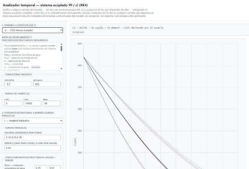
When we want to study the behavior of dynamic variables with memory, we must solve the equations that determine their temporal evolution and graphically represent each variable as a function of time.

Additionally, we can analyze how this evolution changes by modifying one of the forcing and/or structural parameters. To do this, different values of the parameter can be defined and a time curve represented for each one, which allows us to directly visualize its effect on the dynamics of the system.

It is also important to consider the uncertainty associated with the measurements used by the model and estimate how this propagates through the calculations. In this way, in addition to the curve corresponding to the estimated value of the variable, its range of uncertainty can be represented by two dotted lines that delimit the lower and upper expected values:

ID:('gp', 647)

Storyboard

In 1905, Albert Einstein published one of the works that would mark the birth of modern statistical physics. His goal was to demonstrate that the irregular motion observed in small particles suspended in a liquidBrownian motioncould be explained as a direct consequence of random collisions produced by invisible molecules in the fluid. To do this, he developed a mathematical model capable of relating microscopic fluctuations with macroscopic properties measurable in the laboratory.

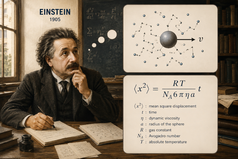
The result was an equation that connects the root mean square displacement of a particle with time, temperature, fluid dynamic viscosity, and particle size. In this relationship, Avogadro's number, $N_A$, appears, establishing a bridge between the microscopic world of atoms and the macroscopic world of experimental measurements. While temperature and viscosity could be determined directly in the laboratory, the value of $N_A$ had not yet been convincingly measured, so the equation offered a completely new method for determining it.

The expression shown in the figure corresponds to the form later used by Jean Perrin to analyze his experiments on Brownian motion. By measuring the displacement of particles suspended in a fluid and knowing the temperature, viscosity and size of these particles, Perrin was able to solve for the value of $N_A$ and compare it with that obtained by completely independent methods.

The importance of this work transcends Brownian motion itself. Einstein did not construct an equation by empirically fitting data, but rather deduced it from fundamental principles of statistical physics. Consequently, all parameters of the equation have a well-defined physical meaning and can be measured independently of the experiment used to validate it. This approach constitutes the ideal of scientific modeling: developing equations based on universal laws of nature, whose parameters represent real physical properties and not simple adjustment constants. It was precisely the experimental confirmation carried out by Perrin that consolidated this vision and transformed Einstein's equation into one of the classic examples of a model based on fundamental principles.

ID:('gp', 658)

Storyboard

In 1905, Albert Einstein developed a theoretical description of Brownian motion that related the random displacement of small particles suspended in a fluid to measurable physical properties such as temperature, viscosity, and particle size. In that equation a fundamental constant appeared, $N_A$, whose physical interpretation had not yet been demonstrated experimentally.

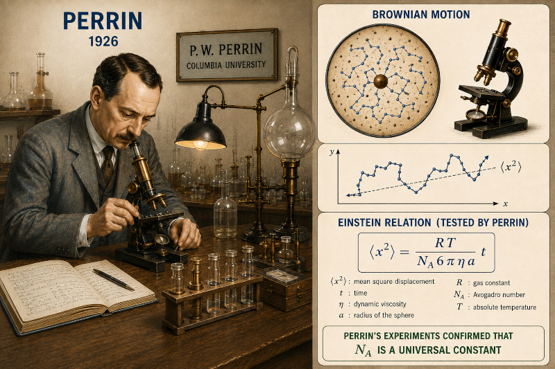
Two decades later, Jean Perrin carried out a series of experiments observing the Brownian motion of tiny particles suspended in a liquid under a microscope. By measuring its mean square displacement and using the relationship proposed by Einstein, he was able to solve for the value of $N_A$. The result coincided with Avogadro's number obtained by completely independent methods, demonstrating that the constant introduced by Einstein effectively corresponded to a universal constant of nature and not to a simple adjustment parameter.

This result had enormous importance for physics. Einstein's equation ceased to be an expression whose validity depended on an experimentally adjusted numerical value and became a law based on fundamental principles, whose parameters have a universal physical meaning. In other words, the theory not only correctly described a particular experiment, but was connected to the fundamental constants that govern all matter.

This joint work by Einstein and Perrin represents an example of the gold standard in scientific modeling. The objective is not to build equations that work only for a specific system through adjusted parameters, but to develop models whose parameters correspond to universal magnitudes of physics and, therefore, can be applied and verified in a wide variety of phenomena. This search for universality is what distinguishes a model based on physical principles from a simple numerical adjustment of data.

ID:('gp', 659)

Storyboard

Not all equations have the same scientific value, even if they can all correctly reproduce a set of experimental data. The difference lies in how they were constructed and, therefore, in their ability to explain a phenomenon, extrapolate to new conditions and reveal the physical mechanisms that govern the system.

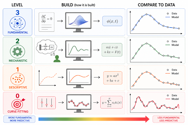
The equations can be classified into four main levels:

• Level 0 Curve Fitting.

The equation is obtained by fitting a mathematical function to a set of experimental data. Its goal is to reproduce observations with as little error as possible, but its parameters usually have no physical meaning. These equations usually describe the data used for fitting well, although their predictive ability outside that range is limited.

• Level 1 Descriptive.

The equation summarizes the observed behavior using a simple mathematical expression, such as a polynomial or an empirical function. Although it describes general tendencies of the system, it does not yet represent the physical mechanisms that generate such behavior.

• Level 2 Mechanistic.

The equation is built from knowledge of the physical, chemical or biological processes involved. Each term represents an identifiable mechanism and the parameters have a specific meaning within the system studied. These models allow us to understand how different processes interact and facilitate the analysis of new scenarios.

• Level 3 Fundamental.

It corresponds to the highest level of modeling. The equation is derived from general physical principles, such as conservation laws, variational principles, or fundamental theories. Its parameters correspond to universal constants or physical properties that are measurable independently of the system analyzed. Therefore, these models have a high predictive capacity and can be applied to a wide variety of phenomena without requiring specific readjustments.

An important feature is that all levels can show excellent agreement with experimental data. However, a good match with measurements does not guarantee that the model correctly represents the physics of the phenomenon. Two equations can fit the same data almost perfectly, but one of them is only a mathematical approximation while the other reflects the fundamental mechanisms that govern the system.

For this reason, in scientific modeling the objective is not only to minimize the error with respect to the data, but to construct equations supported by increasingly general principles. The classic example is the work of Einstein and Perrin: an equation acquires true scientific power when its parameters stop being simple numerical adjustments and begin to represent universal constants of nature. That is the standard to which modeling based on fundamental principles aspires.

ID:('gp', 660)

Storyboard

Just as equations can be classified according to their level of foundation, the variables and parameters that appear in them also have different levels of scientific quality. The main difference lies in how each value is obtained and how independent it is from the model itself. The more universal and independent a parameter is, the greater the predictive capacity of the model and the less need to adjust it each time it is applied to a new system.

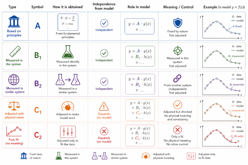
The variables and parameters can be classified into five main categories:

• Category $A$ Based on fundamental principles.

It corresponds to universal constants or parameters derived directly from fundamental laws of physics. Its value does not depend on the particular system being studied or the model used. Typical examples are the speed of light, Planck's constant, Avogadro's number or the gas constant. They constitute the level of highest scientific quality.

• Category $B_1$ Measurement in the system.

They are physical properties determined experimentally in the system to be modeled. Although they are not universal, they do not depend on the mathematical model used. Examples are the viscosity of a fluid, a measured kinetic constant, or the conductivity of a specific material.

• Category $B_2$ Measured in a similar system.

The parameter comes from experiments carried out on an equivalent or sufficiently similar system. It has not been adjusted for the current model, but transferred from another experimental situation. This category allows reusing existing knowledge when direct measurements are not available.

• Category $C_1$ Adjusted with physical meaning.

The parameter must be adjusted for the model to correctly reproduce the data, but this adjustment is done within physically reasonable limits while preserving clear interpretation. After adjustment, the obtained value can be compared with independent measurements or with values expected according to theory.

• Category $C_2$ Purely numerical adjustment.

The parameter exists solely to improve the agreement between the model and the experimental data. It has no independent physical meaning and cannot be measured or verified outside of the model itself. Although these types of parameters usually improve the fit, they also increase the risk of overfitting and considerably reduce the predictive capacity of the model.

This classification allows the quality of a mathematical model to be objectively evaluated. Two models can reproduce a set of experimental data with the same precision, but the one that uses a greater proportion of variables from the categories $A$, $B_1$ and $B_2$ will generally be more robust, more explanatory and more reliable when extrapolating to new conditions. On the other hand, a model that depends mainly on parameters $C_1$ and, especially, $C_2$, can correctly describe the available data, but its ability to predict the behavior of the system outside the fitting conditions will be much lower.

Consequently, one of the central objectives of scientific modeling is to progressively replace the adjusted parameters with variables whose value comes from fundamental principles or independent measurements. Following the ideal set forth by Einstein and experimentally confirmed by Perrin, a good model must not only fit the data, but also be constructed with parameters that have universal or independently verifiable physical meaning.

ID:('gp', 661)