
Rebound in walls orthogonal to the network
Definition 
If the collision does not occur at the point of the network, but at a distance
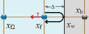
\\n\\nthen the function must consider the offset by weighting the contributions\\n\\n
$f_i(x_f,t+\delta t)=\displaystyle\frac{(1-\Delta)f_{-i}(x_f,t)+\Delta(f_{-i}(x_b,t)+f_{-i}(x_{f2},t)}{1+\Delta}$
ID:(8499, 0)
Rebound on walls with inclination
Image
If the wall shows an inclination with respect to the network it must be modeled in a more complex form:
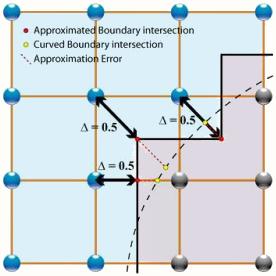
More general edge
First, an approximate boundary must be defined to allow the necessary edge equations to be established. Then they must be applied in the process of steraming.
ID:(8500, 0)
Example of Streaming Equations
Note
In the case of a D2Q9 system we have the 9 values ``` N[x,y] = N[x,y-1] NW[x,y] = NW[x+1,y-1] E[x,y] = E[x-1,y] NE[x,y] = NE[x-1,y-1] S[x,y] = S[x,y+1] SE[x,y] = SE[x-1,y+1] W[x,y] = W[x+1,y] SW[x,y] = SW[x+1,y+1] ```
ID:(9151, 0)
Equation of Propagation
Storyboard
Variables
Calculations
Calculations
Equations
Examples
If the collision does not occur at the point of the network, but at a distance
$f_i(x_f,t+\delta t)=\displaystyle\frac{(1-\Delta)f_{-i}(x_f,t)+\Delta(f_{-i}(x_b,t)+f_{-i}(x_{f2},t)}{1+\Delta}$
If the wall shows an inclination with respect to the network it must be modeled in a more complex form:
More general edge
First, an approximate boundary must be defined to allow the necessary edge equations to be established. Then they must be applied in the process of steraming.
In the streaming process the particles are moved according to their velocity directions to neighboring cells
where
In the case of a D2Q9 system we have the 9 values ``` N[x,y] = N[x,y-1] NW[x,y] = NW[x+1,y-1] E[x,y] = E[x-1,y] NE[x,y] = NE[x-1,y-1] S[x,y] = S[x,y+1] SE[x,y] = SE[x-1,y+1] W[x,y] = W[x+1,y] SW[x,y] = SW[x+1,y+1] ```
ID:(1152, 0)