
Review of the Lattice Boltzmann Method (LBM)
Storyboard
The Lattice Boltzmann Method (LBM) was created to reduce the processing time in the solution of hydro and aerodynamic problems. Instead of solving the Navier Stokes differential equation, it uses an equivalent representation based on the Boltzmann transport equation and reduces the processing effort by working with a simplified discrete phase space. The result is a high-speed simulator capable of describing highly complex processes.
ID:(1162, 0)
Boltzmann equation
Equation
The Boltzmann function describes the transport of a particle system described by the velocity distribution function:
| $\displaystyle\frac{\partial f}{\partial t}+v_i\displaystyle\frac{\partial f}{\partial x_i}=C(f)$ |
Where the term
ID:(8462, 0)
Density
Equation
If the parameters are calculated by averaging over the speed using
| $ \chi_k(\vec{x},t) =\displaystyle\frac{1}{c(\vec{x},t)}\displaystyle\int d\vec{v} f(\vec{x},\vec{v},t) \chi_k(\vec{x},\vec{v},t)$ |
the mass density estimation is obtained by:
| $\rho(\vec{x},t) = m\displaystyle\int f(\vec{x},\vec{v},t)d\vec{v}$ |
ID:(8458, 0)
Speed of the Flow
Equation
If the parameters are calculated by averaging over the speed using
| $ \chi_k(\vec{x},t) =\displaystyle\frac{1}{c(\vec{x},t)}\displaystyle\int d\vec{v} f(\vec{x},\vec{v},t) \chi_k(\vec{x},\vec{v},t)$ |
the velocity of the flow is calculated by integrating the velocity distribution function on all velocities by weighing the velocities:
| $\vec{u}(\vec{x},t) = \displaystyle\frac{m}{\rho}\int \vec{v}f(\vec{x},\vec{v},t)d\vec{v}$ |
ID:(8459, 0)
Temperature
Equation
If the parameters are calculated by averaging over the speed using
| $ \chi_k(\vec{x},t) =\displaystyle\frac{1}{c(\vec{x},t)}\displaystyle\int d\vec{v} f(\vec{x},\vec{v},t) \chi_k(\vec{x},\vec{v},t)$ |
and the equipartition theorem is considered, the temperature can be estimated by integrating the kinetic energy weighted by the velocity distribution divided by the gas constant:
| $T(\vec{x},t) = \displaystyle\frac{m}{3R\rho}\displaystyle\int (\vec{v}\cdot\vec{v})f(\vec{x},\vec{v},t)d\vec{v}$ |
ID:(8460, 0)
Tension tensor
Equation
If the parameters are calculated by averaging over the speed using
| $ \chi_k(\vec{x},t) =\displaystyle\frac{1}{c(\vec{x},t)}\displaystyle\int d\vec{v} f(\vec{x},\vec{v},t) \chi_k(\vec{x},\vec{v},t)$ |
the flow tensor is calculated by integrating the velocity distribution function on all velocities by weighing the velocity differences:
| $\sigma_{ij} = m\displaystyle\int (v_i-u_i)(v_j-u_j)f(\vec{x},\vec{v},t)d\vec{v}$ |
ID:(8461, 0)
Lattice Boltzmann Method
Description
The problem with macro scale systems that are based on microscopic phenomena is that
- macroscopic models are too simple to correctly reflect the dynamics
- microscopic models to describe the macroscopic reality can not be solved analytically and numerical solutions are cumbersome (= require a lot of computational resources)
The Boltzmann lattice method looks for an intermediate path. It is based on the Boltzmann transport equation, rescues the microscopic part via the collision term and implements a simplified structure to calculate the macroscopic results. We speak of a mesoscopic approach where we can, as required, reduce microscopic effort by losing accuracy but saving resources or improving accuracy by investing more resources.
ID:(8488, 0)
D2Q9 Models (2 dimensions, 9 points)
Image
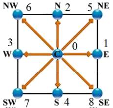
El modelo D2Q9 es un modelo bidimensional (D2) en que se se conecta el nodo (punto central) en nodos a lo largo de los ejes cartesianos\\n\\nen el origen\\n\\n
$\vec{e}_0=(0,0)$
\\n\\nen las esquinas\\n\\n
$\vec{e}_1=(1,0)$
(E),\\n
$\vec{e}_2=(0,1)$
(N), \\n
$\vec{e}_3=(-1,0)$
(W) y \\n
$\vec{e}_4=(0,-1)$
(S)\\n\\ny en las diagonales\\n\\n
$\vec{e}_5=(1,1)$
(NE), \\n
$\vec{e}_6=(-1,1)$
(SE), \\n
$\vec{e}_7=(-1,-1)$
(SW) y \\n
$\vec{e}_8=(1,-1)$
(NW)
lo que se representa en la siguiente gráfica:
ID:(8496, 0)
D3Q15 Models (3 dimensions, 15 points)
Image
The D3Q15 model is a two-dimensional model (D3) in which the node (central point) is connected in nodes along Cartesian axes\\n\\n
$(1,0,0), (-1,0,0), (0,1,0), (0,-1,0), (0,0,1) (0,0,-1)$
\\n\\nand in the corners of the bucket\\n\\n
$(1,0,1), (-1,0,1), (0,1,1) , (0,-1,1), (1,0,-1), (-1,0,-1), (0,1,-1) , (0,-1,-1)$
which is represented in the following graph:
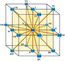
It is easy to build models of type D3Q19 (including side edge halves) or D3Q27 (all possible points).
ID:(8497, 0)
Discretization function
Equation
In the case of the discretization in the LBM models we work not with functions of the speed if not with discrete components. In this way the
| $f_i(\vec{x},t)=w_if(\vec{x},\vec{v}_i,t)$ |
where
ID:(8466, 0)
Streaming
Equation
In the streaming process the particles are moved according to their velocity directions to neighboring cells
| $f_i(\vec{x},t)\leftarrow f_i(\vec{x}+ce_i\delta t,t+\delta t)$ |
where
ID:(9150, 0)
Rebound in walls orthogonal to the network
Image
If the collision does not occur at the point of the network, but at a distance
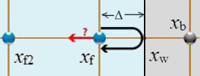
\\n\\nthen the function must consider the offset by weighting the contributions\\n\\n
$f_i(x_f,t+\delta t)=\displaystyle\frac{(1-\Delta)f_{-i}(x_f,t)+\Delta(f_{-i}(x_b,t)+f_{-i}(x_{f2},t)}{1+\Delta}$
ID:(8499, 0)
Rebound on walls with inclination
Image
If the wall shows an inclination with respect to the network it must be modeled in a more complex form:
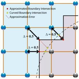
More general edge
First, an approximate boundary must be defined to allow the necessary edge equations to be established. Then they must be applied in the process of steraming.
ID:(8500, 0)
Example of Streaming Equations
Description
In the case of a D2Q9 system we have the 9 values ``` N[x,y] = N[x,y-1] NW[x,y] = NW[x+1,y-1] E[x,y] = E[x-1,y] NE[x,y] = NE[x-1,y-1] S[x,y] = S[x,y+1] SE[x,y] = SE[x-1,y+1] W[x,y] = W[x+1,y] SW[x,y] = SW[x+1,y+1] ```
ID:(9151, 0)
Ejemplo de elemento de Colisión
Description
In case D2Q9 the term collision is calculated by summing the different factors
| $f_i^{eq}=\rho\omega_i\left(1+\displaystyle\frac{3\vec{u}\cdot\vec{e}_i}{c}+\displaystyle\frac{9(\vec{u}\cdot\vec{e}_i)^2}{2c^2}-\displaystyle\frac{3u^2}{2c^2}\right)$ |
so you have for each cell
```
O = O+w(4rho/9)(1-3u2/2) - O)
E = E+w(rho/9)(1 + u_x/3+5u_x^2-3u2/2)-E)
W = W+w(rho/9)(1 - u_x/3+5u_x^2-3u2/2)-W)
N = N+w(rho/9)(1 + u_y/3+5u_y^2-3u2/2)-N)
S = S+w(rho/9)(1 - u_y/3+5u_y^2-3u2/2)-S)
NE = NE+w(rho/36)(1+u_x/3+u_y/3+5(u2+2u_xu_y)/2-3u2/2) - NE)
SE = SE+w(rho/36)(1+u_x/3-u_y/3+5(u2-2u_xu_y)/2-3u2/2) - SE)
NW = NW+w(rho/36)(1-u_x/3+u_y/3+5(u2-2u_xu_y)/2-3u2/2) - NW)
SW = SW+w(rho/36)(1-u_x/3-u_y/3+5(u2+2u_xu_y)/2-3u2/2) - SW)
```
with
```
u2 = u_x^2+u_y^2
```
ID:(9155, 0)
LBM equation in the relaxation approximation
Equation
In the relaxation approximation, it is assumed that the distribution
$\displaystyle\frac{df_i}{dt}=-\displaystyle\frac{f_i-f_i^{eq}}{\tau}$
which has in the discrete approximation the equation
| $f_i(\vec{x}+c\vec{e_i}\delta t,t+\delta t)=f_i(\vec{x},t)+\displaystyle\frac{1}{\tau}(f_i^{eq}(\vec{x},t)-f_i(\vec{x},t))\delta t$ |
where the term of the differences in the distribution functions represents the collisions.
ID:(8489, 0)
Distribution in Balance (Gas of Particles)
Equation
The equilibrium distribution can be approximated by a distribution of Maxwell Boltzmann
| $f_i^{eq}=\displaystyle\frac{m}{2\pi kT}e^{-m|c\vec{e}_i-\vec{u}|^2/2kT}$ |
Where
ID:(8490, 0)
Bhatnagar-Gross-Krook Approach
Equation
En la aproximación Bhatnagar-Gross-Krook la distribución en equilibrio se asume como la de un gas de partículas sin interacción
| $f^{(0)}(\vec{x},\vec{v},t)=c(\vec{x},t)\left(\displaystyle\frac{m\beta}{2\pi}\right)^{3/2}e^{-\beta m(\vec{v}-\vec{u}(\vec{x},t))^2/2}$ |
con
| $f_i^{eq}=\rho\omega_i\left(1+\displaystyle\frac{3\vec{u}\cdot\vec{e}_i}{c}+\displaystyle\frac{9(\vec{u}\cdot\vec{e}_i)^2}{2c^2}-\displaystyle\frac{3u^2}{2c^2}\right)$ |
con
| Modelo | $\omega_i$ | Index |
| 1DQ3 | ? | i=0 |
| - | ? | i=1, 2 |
| 2DQ9 | 4/9 | i=0 |
| - | 1/9 | i=1,...,4 |
| - | 1/36 | i=5,...,8 |
| 3DQ15 | 1/3 | i=0 |
| - | 1/18 | i=1,...,6 |
| - | 1/36 | i=7,...,14 |
| 3DQ19 | ? | i=0 |
| - | ? | i=1,...,6 |
| - | ? | i=7,...,18 |
que se determinan asegurando que la distribución equilibrio cumpla las leyes de conservación.
ID:(9084, 0)
Example Hydrodynamic Simulator
Description
In the case of particles of a liquid, the method LBM allows to develop simulators as shown in the example:
ID:(9156, 0)