
Balance Equation Solution
Storyboard
The equations for the temperature of the earth's surface, bottom and top of the atmosphere can be solved by disturbance techniques. This is assumed small variations in solar intensity, albedos and coverage factors and it is estimated how these affect the variation of these temperatures.
ID:(575, 0)
New earth temperature
Equation
The new temperature $T_{et}$ is calculated by adding the initial temperature $T_e$ with the variation $\delta T_e$:
ID:(7605, 0)
New lower atmosphere temperature
Equation
The new temperature $T_{bt}$ is calculated by adding the initial temperature $T_b$ with the variation $\delta T_b$:
ID:(7606, 0)
New upper atmosphere temperature
Equation
The new temperature $T_{tt}$ is calculated by adding the initial temperature $T_t$ with the variation $\delta T_t$:
ID:(7607, 0)
Fundamentals of the model
Description
Since the parameters of the model vary little around their mean values, a Taylor expansion can be performed around the mean values. This yields linear equations that can be solved exactly.
ID:(84, 0)
New intensity
Equation
The new intensity $I_{st}$ is calculated by adding the initial intensity $I_s$ with the variation $\delta I_s$:
ID:(7604, 0)
Basic model of radiative flux
Image
The following diagram illustrates the main radiative fluxes (visible and infrared) in a simplified Earth model:
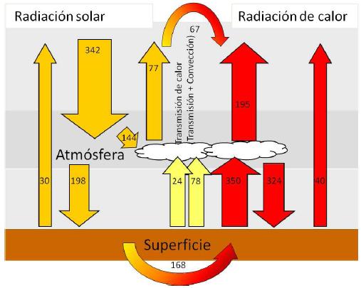
This diagram represents, in a simplified manner, the interaction of radiation on Earth. Visible radiation from the sun reaches the Earth\'s surface, where it can be reflected back into space, absorbed by the Earth\'s surface and converted into infrared radiation, or absorbed by the atmosphere. In turn, the Earth emits infrared radiation into space.
These radiative fluxes are fundamental to understanding the energy balance of our planet and the processes that regulate climate.
ID:(7331, 0)
Assumption evolution of society
Description
To simulate the future development of climate, four possible scenarios were assumed:
- A1: Rapid economic growth, energy consumption triples by 2100. Population increase to 9 billion by 2050 and subsequent slow decline.
- A2: Moderate economic growth, energy consumption increases gradually but triples by 2100. Continuous population increase to 15 billion by 2100.
- B1: Rapid economic growth, energy consumption decreases by 2100. Population increase to 9 billion by 2050 and subsequent slow decline.
- B2: Slower economic growth, energy consumption increases significantly but stabilizes by 2100. Slow population increase to 10 billion by 2100.
For each of these scenarios, the following are estimated:
- Energy consumption and the way it is generated.
- Production and type of food consumed.
Additionally, the generation of corresponding gases is estimated.
ID:(7324, 0)
Balance Equations
Description
In the case of equilibrium, the following three radiative equilibrium equations hold:
$(1 - a_a)(1 - \gamma_{\nu})I_s - \kappa (T_e - T_b) - \sigma\epsilon_eT_e^4 + \sigma\epsilon_b T_b^4 = 0$
$\kappa(T_e - T_b) + \gamma_i\sigma\epsilon_e T_e^4 - 2\sigma\epsilon_bT_b^4 = 0$
$(1 - a_a)\gamma_{\nu} + \sigma\epsilon_b T_b^4 - 2\sigma\epsilon_t T_t^4 = 0$
where $T_e$ is the temperature of the Earth, $T_b$ is the temperature of the lower atmosphere, and $T_t$ is the temperature of the upper atmosphere. Additionally, we have the average solar radiation $I_s$, the albedos of the atmosphere and Earth denoted by $a_a$ and $a_e$ respectively, $\gamma_{
u}$ and $\gamma_i$ representing the coverage factors in the visible and infrared range, $\epsilon_e$ and $\epsilon_a$ representing the emissivity of Earth and the atmosphere, and $\sigma$ as the Stefan-Boltzmann constant.
ID:(85, 0)
Approximate Equations
Description
Using the approximations, we obtain for the equation that in a linear approximation is:
$-\kappa(\delta T_e-\delta T_b)-4\sigma\epsilon_e T_e^3\delta T_e+4\sigma\epsilon_b T_b^3\delta T_b-\delta a_e(1-\gamma_{\nu})I_s-(1-a_e)\delta\gamma_{\nu}I_s=0$
Similarly, for the second equation, we have:
$\kappa(\delta T_e-\delta T_b)+\sigma\epsilon_e T_e^4\delta\gamma_i+4\gamma_i\sigma\epsilon_e T_e^3\delta T_e+4\sigma\epsilon_t T_t^3\delta T_t-8\sigma\epsilon_b T_b^3\delta T_b=0$
And for the third equation:
$-2\sigma \epsilon_t T_t^3\delta T_t+\sigma\epsilon_b T_b^3\delta T_b-\gamma_{\nu}I_s\delta a_a+(1-a_a) I_s\delta\gamma_i=0$
These three equations form a system of linear equations to calculate the variations of the temperatures $\delta T_e$, $\delta T_b$, and $\delta T_t$ in terms of the variations of the albedos $\delta a_e$ and $\delta a_a$, and the coverage factors $\delta \gamma_{
u}$ and $\delta \gamma_i$.
ID:(87, 0)
Model simulator
Description
The radiative balance equations allow us to calculate the temperatures on the Earth\'s surface $T_e$, in the lower atmosphere $T_b$, and at the top $T_t$. These equations are represented as follows:
Equation 1: The change in temperature at the Earth\'s surface is calculated using the equation:
$M_eC_e\displaystyle\frac{dT_e}{dt}=(1-a_e)(1-\gamma_v)I_s-\kappa(T_e-T_b)-\sigma\epsilon T_e^4+\sigma\epsilon T_b^4$
where $M_e$ is the mass of the Earth, $C_e$ is the heat capacity of the Earth, $a_e$ is the Earth\'s albedo, $\gamma_v$ is the fraction of visible radiation absorbed by the atmosphere, $I_s$ is the incident solar radiation, $\kappa$ is the thermal conductivity, $\sigma$ is the Stefan-Boltzmann constant, and $\epsilon$ is the emissivity of the Earth.
Equation 2: The change in temperature in the lower atmosphere is calculated using the equation:
$M_bC_b\displaystyle\frac{dT_b}{dt}=\kappa(T_e-T_b)+\gamma_i\sigma\epsilon T_e^4-2\sigma\epsilon T_b^4+\sigma\epsilon T_t^4=0$
where $M_b$ is the mass of the atmosphere, $C_b$ is the heat capacity of the atmosphere, and $\gamma_i$ is the fraction of infrared radiation absorbed by the atmosphere.
Equation 3: The change in temperature at the top of the atmosphere is calculated using the equation:
$M_tC_t\displaystyle\frac{dT_t}{dt}=(1-a_a)\gamma_vI_s+\sigma\epsilon T_b^4-2\sigma\epsilon T_t^4=0$
where $M_t$ is the mass of the upper atmosphere and $C_t$ is the heat capacity of the upper atmosphere.
These equations represent the balance between incident solar radiation, radiation emitted by the Earth, and radiation transferred between different layers of the Earth and the atmosphere. By solving these equations, we can obtain the temperatures in each of these layers.
ID:(6867, 0)
Numerical solution
Description
The system of equations can be solved analytically. If we evaluate the expressions for the parameters of the current Earth condition ($a_e = 0.152$, $a_a = 0.535$, $\gamma_{
u} = 0.421$, $\gamma_i=0.897$, $\kappa = 2.226 , \text{W/m}^2\text{K}^{-1}$, $\epsilon_e = \epsilon_b = \epsilon_t = 1$, $I_s = 342 , \text{W/m}^2$, $T_e = 14.8^\circ \text{C}$, $T_b = 1.79^\circ \text{C}$, and $T_t = -30.98^\circ \text{C}$), we would have:
| $\delta T_e = 0.240\delta I_s - 97.978\delta\gamma_v+123.671\delta \gamma_i - 84.112\delta a_e - 22.827\delta a_a$ |
| $\delta T_b = 0.193\delta I_s - 66.120\delta \gamma_v + 136.209\delta \gamma_i - 64.106\delta a_e - 25.142\delta a_a$ |
| $\delta T_t = 0.172\delta I_s - 23.693\delta \gamma_v + 99.662\delta \gamma_i-46.905\delta a_e - 40.745\delta a_a$ |
ID:(7319, 0)
Solución numérica, Temperatura terrestre
Equation
La temperatura terrestre se puede estimar mediante:
$\delta T_e = 0.240\delta I_s - 97.978\delta\gamma_{
u}+123.671\delta \gamma_i - 84.112\delta a_e - 22.827\delta a_a$
$\delta T_b = 0.193\delta I_s - 66.120\delta \gamma_{
u} + 136.209\delta \gamma_i - 64.106\delta a_e - 25.142\delta a_a$
$\delta T_t = 0.172\delta I_s - 23.693\delta \gamma_{
u} + 99.662\delta \gamma_i-46.905\delta a_e - 40.745\delta a_a$
donde se asumieron los valores
Parámetros | Valor
-------------------|:---------:
$a_e$ | $0.152$
$a_a$ | $0.535$
$\gamma_{
u}$ | $0.421$
$\gamma_i$ | $0.897$
$\kappa$ | $2.226W/m^2K$
$\epsilon_e$ | $1$
$\epsilon_b$ | $1$
$\epsilon_t$ | $1$
$I_s$ | $342W/m^2$
$T_e$ | $14.8^{\circ}C$
$T_b$ | $1.79^{\circ}C$
$T_t$ | $-30.98^{\circ}C$
ID:(7440, 0)
Solución numérica, Temperatura atmosferica (inferior)
Equation
La temperatura terrestre se puede estimar mediante:
$\delta T_e = 0.240\delta I_s - 97.978\delta\gamma_{
u}+123.671\delta \gamma_i - 84.112\delta a_e - 22.827\delta a_a$
$\delta T_b = 0.193\delta I_s - 66.120\delta \gamma_{
u} + 136.209\delta \gamma_i - 64.106\delta a_e - 25.142\delta a_a$
$\delta T_t = 0.172\delta I_s - 23.693\delta \gamma_{
u} + 99.662\delta \gamma_i-46.905\delta a_e - 40.745\delta a_a$
donde se asumieron los valores
Parámetros | Valor
-------------------|:---------:
$a_e$ | $0.152$
$a_a$ | $0.535$
$\gamma_{
u}$ | $0.421$
$\gamma_i$ | $0.897$
$\kappa$ | $2.226W/m^2K$
$\epsilon_e$ | $1$
$\epsilon_b$ | $1$
$\epsilon_t$ | $1$
$I_s$ | $342W/m^2$
$T_e$ | $14.8^{\circ}C$
$T_b$ | $1.79^{\circ}C$
$T_t$ | $-30.98^{\circ}C$
ID:(7441, 0)
Solución numérica, Temperatura atmosferica (superior)
Equation
La temperatura terrestre se puede estimar mediante:
$\delta T_e = 0.240\delta I_s - 97.978\delta\gamma_{
u}+123.671\delta \gamma_i - 84.112\delta a_e - 22.827\delta a_a$
$\delta T_b = 0.193\delta I_s - 66.120\delta \gamma_{
u} + 136.209\delta \gamma_i - 64.106\delta a_e - 25.142\delta a_a$
$\delta T_t = 0.172\delta I_s - 23.693\delta \gamma_{
u} + 99.662\delta \gamma_i-46.905\delta a_e - 40.745\delta a_a$
donde se asumieron los valores
Parámetros | Valor
-------------------|:---------:
$a_e$ | $0.152$
$a_a$ | $0.535$
$\gamma_{
u}$ | $0.421$
$\gamma_i$ | $0.897$
$\kappa$ | $2.226W/m^2K$
$\epsilon_e$ | $1$
$\epsilon_b$ | $1$
$\epsilon_t$ | $1$
$I_s$ | $342W/m^2$
$T_e$ | $14.8^{\circ}C$
$T_b$ | $1.79^{\circ}C$
$T_t$ | $-30.98^{\circ}C$
ID:(7442, 0)
Calentamiento Global bajo distintos escenarios
Image
Si se consideran los distintos escenarios B1, A1B y A1 se puede estudiar la probable evolución de la temperatura sobre la superficie del planeta.
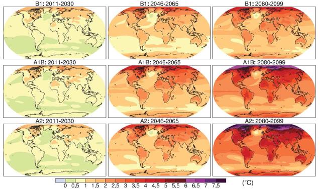
Calentamiento Global bajo distintos escenarios
| Escenarios | 1990 | A1FI | A1B | A1T | A2 | B1 | B2 |
| Población (1E+9) | 5.3------|||||||
| 2020 | -7.67.57.68.27.67.6|||||||
| 2050 | -8.78.78.711.38.79.3|||||||
| 2100 | -7.17.17.015.17.010.4|||||||
| GDP (1E+12 1990US$/yr) | 21------|||||||
| 2020 | -535657415351|||||||
| 2050 | -16418118782136110|||||||
| 2100 | -525529550243328235|||||||
| CO2, fosil (GtC/yr) | 6.0------|||||||
| 2020 | -11.212.110.011.010.09.0|||||||
| 2050 | -23.116.012.316.511.711.2|||||||
| 2100 | -30.313.14.328.95.213.8|||||||
| CO2, agro (GtC/yr) | 1.1------|||||||
| 2020 | -1.50.50.31.20.60.0|||||||
| 2050 | -0.80.40.00.9-0.4-0.2|||||||
| 2100 | --2.10.40.00.2-1.0-0.5|||||||
| Metano, (MtCH4/yr) | 310------|||||||
| 2020 | -416421415424377384|||||||
| 2050 | -630452500598359505|||||||
| 2100 | -735289274889236597|||||||
| NO, (MtN/yr) | 6.7------|||||||
| 2020 | -9.37.26.19.68.16.1|||||||
| 2050 | -14.57.46.112.08.36.3|||||||
| 2100 | -16.67.05.416.55.76.9
ID:(7333, 0)
Calentamiento Global (ejemplo)
Image
La siguiente gráfica muestra el calentamiento según zona geográfica:
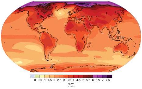
Calentamiento Global (ejemplo)
ID:(7332, 0)