
 User:
User:


Equations and Variables
Storyboard

Following the guideline presented at the end of this section, a textual description of the system is written, avoiding including equations and the symbology of the variables, but explicitly preserving the physical concepts and causal relationships that these variables represent. From this description, the first prompt allows the artificial intelligence to identify the thematic groups, the concepts involved and the actions or processes that relate them. With this information it builds a semantic network that represents the conceptual functioning of the model. This network constitutes the first stage of validation, since it allows us to verify that the artificial intelligence has correctly interpreted the hypothesis and logic of the system before starting the mathematical formulation. An incorrect conceptual understanding at this stage will inevitably result in an inconsistent set of equations, so this verification is essential for the rest of the modeling process.
ID:('ky', 1792)
Promp for logical network
Storyboard
Once the semantic network of the model has been generated, the next step is to describe in detail each of the thematic groups that will later be represented by their corresponding equations. If the prompt shown below is executed within the same dialog, so that the AI can consult the previously generated group descriptions, the system builds the logical network of the model and automatically generates the list of equations and the associated variables:
ID:('gp', 625)
Logical network of water transport
Storyboard
When you run the prompt in an AI, you obtain the logical network of the model, which shows the identified equations and the variables on which each one depends. The diagram can be scrolled and scaled as a whole, while each node can be moved independently. Below is a non-interactive image for reference:
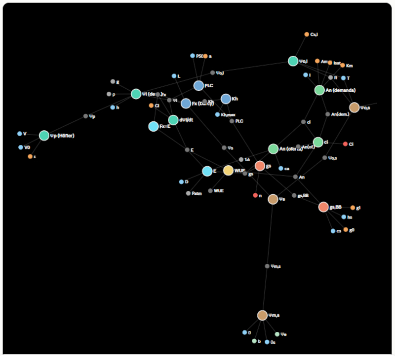
The system also provides the list of equations, indicating for each one its name, mathematical expression, level of reliability, description and origin.
It also generates the list of variables, including their symbol, description, category, category justification and corresponding unit.
Finally, a statistical summary is presented with the distribution of the equations according to their level of reliability and the variables according to their category, providing a global vision of the quality and composition of the generated model.
ID:('gp', 626)
Model equations
Storyboard
The system also provides the list of equations, indicating for each one its name, mathematical expression, level of reliability, description and origin:
ID:('gp', 627)
A problem before creating the simulator
Storyboard
Debugging the model before building the simulator
When developing a complex model, it is common to first build each thematic group of equations independently and then integrate them into a single system. Although each group may be consistent on its own, when connecting them, logical, mathematical, or implementation inconsistencies may appear that are not evident during individual development. For this reason, before generating the simulator it is advisable to carry out a systematic review of the complete model and manually correct any problems detected.
The main types of inconsistencies that can appear are summarized in the following figure and described in more detail in subsequent sections. The prompt that automates this review, identifies the equations and variables involved and proposes alternatives to solve each problem is also presented below.
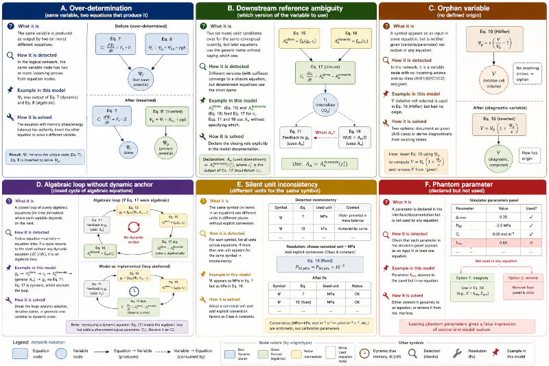
The problems reviewed by the analysis are:
A. Over-determination. The same variable is calculated by two or more different equations, producing a conflict over which of them has the authority to define its value.
B. Downstream reference ambiguity. There are several valid versions of the same physical quantity, but the subsequent equations use the generic name without indicating which of them should be used.
C. Orphan variable. A variable is used as an input to an equation, but it does not have a defined origin: it is not an external input nor is it calculated by any other equation.
D. Algebraic loop without dynamic anchoring. A set of equations forms a closed cycle of algebraic dependencies that prevents calculating the variables in a sequential order without solving the system simultaneously.
E. Silent inconsistency of units. The same symbol, or variables that are combined in an equation, appear expressed with different units without there being an explicit conversion between them.
F. Phantom parameter. A parameter appears in the simulator interface or in the documentation, but no model equation actually uses it, generating a false perception of the model's adjustability.
ID:('gp', 657)
Promp for model review
Storyboard
Before generating the simulator, it is essential to debug the model and correct any possible inconsistencies that it may still contain. The following prompt performs a systematic review of the set of equations, variables and parameters to detect problems such as overdetermination, orphan variables, algebraic loops, unit inconsistencies, ghost parameters and other failures that may affect the operation or interpretation of the model. For each problem encountered, identify the equations and variables involved and propose one or more alternatives to solve it.
Running this prompt is a fundamental step before building the simulator, as it ensures that the model is logically and physically consistent.
Important: execute this prompt in the same chat where the previous prompts were executed, so that the artificial intelligence preserves all the context of the already built model. Then copy and run the following prompt:
ID:('gp', 656)
Over-determination: Two Equations Producing the Same Variable
Storyboard
A model becomes over-determined when the same variable is produced independently by more than one equation, without any explicit hierarchy indicating which equation has authority over that variable. In a logical equation network, this situation appears as a variable node receiving two or more incoming links from different equation nodes. Detecting this condition is simple by grouping the equations according to their output variable: if the same symbol is the target of multiple equations, the model contains an over-determination conflict.
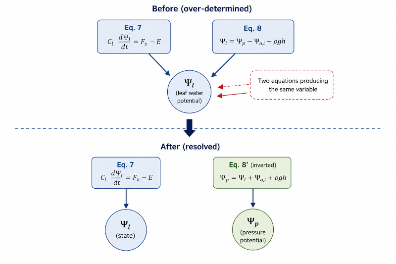
The figure illustrates this situation using the leaf water potential, $\Psi_l$. In the original formulation, both the dynamic balance equation (Eq. 7) and the algebraic water-potential relation (Eq. 8) produce the same variable. As a result, the logical network contains two competing definitions for $\Psi_l$, making it unclear which equation should determine its value during simulation.
The resolution is not to average or combine the equations, but to determine which one represents the true causal mechanism. In physical models, the equation containing a time derivative normally has priority because it describes how the system evolves through time by integrating a conservation law or dynamic balance. The algebraic equation generally expresses an instantaneous physical relationship and therefore should not define the state variable itself.
In this example, Eq. 7 remains the unique equation responsible for computing the state variable $\Psi_l$. The algebraic relation is then inverted so that it computes the pressure potential $\Psi_p$ from the already known value of $\Psi_l$. After this transformation, every variable has a single producer, the logical network becomes unambiguous, and the model preserves both its physical interpretation and its causal consistency.
ID:('gp', 648)
Downstream Reference Ambiguity: Which Version of a Variable Should Be Used?
Storyboard
A different type of inconsistency appears when a model generates multiple valid representations of the same conceptual quantity and later equations refer only to the generic variable name without specifying which version they require. Unlike over-determination, there is no competition between equations attempting to produce the same output. Instead, several candidate variables coexist legitimately, but the downstream model becomes ambiguous because the intended reference is left unspecified.
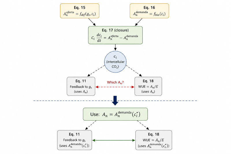
The figure illustrates this situation using the net assimilation rate $A_n$. The diffusive formulation (Eq. 15) computes the supply-limited assimilation, while the biochemical formulation (Eq. 16) computes the demand-limited assimilation. Both quantities are combined by the closure equation (Eq. 17), which determines the equilibrium intercellular $CO_2$ concentration $c_i$. The ambiguity arises because later equations, such as the stomatal feedback (Eq. 11) and the water-use efficiency calculation (Eq. 18), refer simply to $A_n$ without indicating whether they require the supply-limited or the demand-limited value.
This situation can be detected by searching for variables that exist in multiple qualified formssuch as _supply, _demand, _theoretical, or _effectiveand verifying whether downstream equations later use only the unsuffixed symbol. The logical network reveals that the closure equation resolves the relationship between the candidate variables, but the subsequent references fail to identify which resolved quantity should propagate through the remainder of the model.
The ambiguity is removed by explicitly documenting the closure rule rather than leaving it implicit in the implementation. In this model, the downstream variable is defined as the biochemical assimilation evaluated at the equilibrium intercellular $CO_2$ concentration, that is, $A_nA_n$ demand ($c_i$), where $c_i$ is the solution produced by the closure equation. This definition guarantees that every downstream equation uses the same physical quantity and prevents inconsistent interpretations during transient simulations. If the system has not yet reached equilibrium because $c_i$ evolves dynamically, choosing the supply-limited assimilation instead would produce a different value of water-use efficiency and other derived quantities. Consequently, the choice is a fundamental modeling decision rather than a cosmetic naming convention.
ID:('gp', 649)
Orphan Variables: Inputs Without a Defined Origin
Storyboard
An orphan variable is a symbol that is used as an input by one or more equations but has no defined origin within the model. It is neither classified as an external input or parameter nor computed as the output of another equation. As a result, the logical dependency graph contains a variable whose value is required but whose source is undefined, leaving an incomplete causal chain.
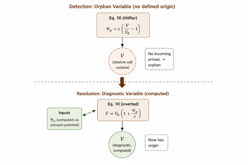
This situation can be detected by examining every variable in the model and verifying whether it belongs to one of two categories: a formally declared input (parameter or measured variable) or the output of an equation. If neither condition is satisfied, the variable is orphaned. In the logical network, it appears immediately as a variable node with no incoming arrows and without the visual classification assigned to known inputs or computed quantities.
The figure illustrates this problem with the relative cell volume $V$. In the original formulation, the Höfler equation uses $V$ as an input to compute the pressure potential $\Psi_p$, while the model itself provides no mechanism explaining where V originates. Although initially classified as a measurable input, relative cell volume is not an environmental quantity that is normally prescribed throughout a simulation. Instead, it is a consequence of the leaf water status and therefore belongs naturally within the model's causal structure.
There are two valid ways to resolve an orphan variable, but one must be selected explicitly. If the variable is genuinely an externally measured or assumed quantity, it should be formally documented as such in the variable classification, together with its justification. In that case, the variable ceases to be orphaned because its origin is explicitly defined by the model documentation. If, however, the variable is actually diagnostic, the appropriate solution is to derive it from existing state variables. In this example, the Höfler relationship is inverted after the pressure potential has been computed, yielding $V=V_0 (1+\Psi_p/\epsilon$). The relative cell volume then becomes a computed diagnostic quantity rather than an assumed input, restoring a complete and consistent causal network.
ID:('gp', 650)
Algebraic Loops Without a Dynamic Anchor
Storyboard
An algebraic loop occurs when a group of equations forms a closed dependency cycle in which every variable depends on another variable within the same loop, and none of the equations contains a time derivative. Such a system has no natural evaluation order because no variable can be computed before the others. Instead, all variables in the cycle must be solved simultaneously or through an iterative numerical procedure.
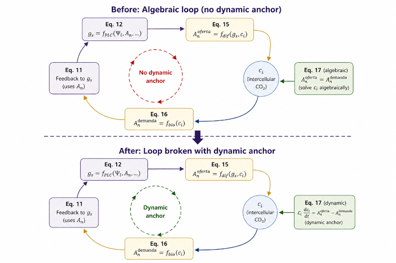
The logical equation network provides a simple way to detect this problem. By following the sequence of equation and variable nodes, any closed path that returns to its starting point without passing through a dynamic equation containing a time derivative represents an algebraic loop. The interactive network makes these situations visually apparent because the variables and equations form a closed ring with no dynamic state acting as a temporary anchor.
The figure illustrates this situation using the $CO_2$ exchange subsystem. The stomatal conductance determines the supply-limited assimilation, which influences the intercellular $CO_2$ concentration, which in turn determines the demand-limited assimilation that feeds back to stomatal conductance. If the closure equation computes the intercellular $CO_2$ concentration purely algebraically by enforcing the equality between supply and demand, the entire subsystem becomes a purely algebraic cycle with no variable possessing temporal memory.
The solution adopted in this model is to transform the closure equation into a dynamic balance by introducing the differential equation for the intercellular $CO_2$ concentration. The state variable $c_i$ then evolves toward equilibrium instead of being solved instantaneously, providing the temporal anchor that breaks the algebraic loop. Although this approach introduces an additional relaxation parameter representing the characteristic response time of the intercellular $CO_2$ concentration, it converts the closed algebraic cycle into a well-defined dynamic system that can be integrated sequentially in time.
More generally, three strategies exist for solving algebraic loops. The preferred solution is to derive a closed analytical solution whenever the equations allow it. When this is impractical, the model documentation should explicitly state that the equations are solved iteratively within each simulation time step, including the convergence criterion and stopping conditions. A third alternative, illustrated here, is to promote one variable in the loop to a dynamic state with a short relaxation time. This introduces a phenomenological parameter that serves primarily as a numerical device rather than as a direct physiological mechanism, and therefore its role should be explicitly documented rather than treated as an implicit modeling assumption.
ID:('gp', 651)
Silent Unit Inconsistencies
Storyboard
A silent unit inconsistency occurs when the same symbol, or two symbols that are added or equated within an equation, are expressed in different physical units across the model without an explicit conversion. Because the symbol name remains unchanged, the inconsistency is often overlooked during model development, even though it introduces numerical errors and compromises the physical interpretation of the equations.
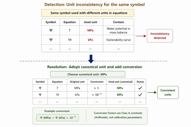
This problem can be detected by examining every occurrence of each variable throughout the equation network and collecting the units associated with that symbol. If the same symbol appears with multiple declared units and no intermediate conversion equation exists, the model contains a unit inconsistency. The same verification should also be applied to quantities that are directly added or equated, since these operations are only physically meaningful when all participating terms share identical dimensions and units.
The figure illustrates this situation using the water potential symbol $\Psi$. In one equation the variable is expressed in megapascals (MPa), while in another it is represented in kilopascals (kPa). Although both quantities describe the same physical property, their numerical values differ by three orders of magnitude. Without an explicit conversion, the model silently mixes incompatible values while preserving identical notation, making the error difficult to detect through visual inspection alone.
The appropriate solution is to adopt a single canonical unit for every physical symbol throughout the entire model. Any equation using a different unit should include an explicit conversion factor before the variable is used. These conversion factors are purely arithmetic relationships and therefore belong to Class A constants, not to calibration parameters such as $C1$ or $C2$. For example, if megapascals are selected as the canonical unit, every occurrence expressed in kilopascals should be converted according to $\psi MPa =\Psi kPa ×10^{3}$. By enforcing one canonical unit for each symbol and documenting every conversion explicitly, the logical consistency of the model is preserved while eliminating a common source of hidden numerical errors.
ID:('gp', 652)
Ghost Parameters: Declared but Never Used
Storyboard
A ghost parameter is a symbol that appears in the simulator interface or in the model documentation but is never actually consumed by any equation. Although the parameter is presented to the user as an adjustable input, modifying its value has no effect on the model because it is disconnected from the computational structure. This creates the false impression that the model contains more controllable physiological mechanisms than it actually does.
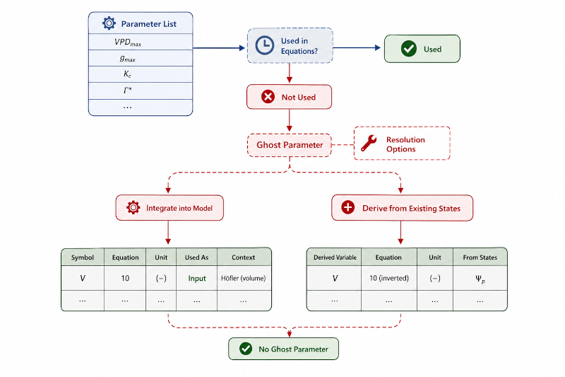
Ghost parameters can be detected by comparing the parameter list with the equation network. Every parameter exposed in the simulator should appear as an input to at least one equation. If a parameter does not occur anywhere in the equation set, it has no computational role and is therefore classified as a ghost parameter. This verification is simple because the logical dependency graph explicitly records every input used by each equation.
The figure illustrates the verification process. Each parameter declared is checked against the equation database to determine whether it is consumed by the model. Parameters that are connected to one or more equations remain valid model inputs. In contrast, parameters that are never referenced are immediately identified as ghost parameters because no computational path links them to the model states or outputs.
There are only two legitimate ways to resolve this situation. If the parameter was intended to influence the system but its connection was omitted during model development, it should be integrated explicitly into the appropriate equation so that its effect becomes part of the causal structure. Alternatively, if the parameter is not required by the model, it should be removed from the simulator interface and from the documentation. A third possibility, when appropriate, is to recognize that the quantity is not an independent parameter at all but rather a diagnostic variable that can be derived from existing state variables, as illustrated in the figure.
Removing ghost parameters is more than a matter of software maintenance. Parameters represent the degrees of freedom that a user believes can influence the simulated system. Displaying parameters that have no computational effect overstates the explanatory and predictive capabilities of the model and compromises its epistemic transparency. Ensuring that every exposed parameter participates in at least one equation guarantees that the simulator faithfully represents the underlying mathematical model.
ID:('gp', 653)
Promp to generate logical network and debugged tables
Storyboard
Once the necessary corrections to eliminate the inconsistencies in the initial model have been defined, it is necessary to regenerate the logic network, the set of equations, and the list of variables so that they all reflect the corrected version of the model. To do this, you can use an artificial intelligence model by running the following prompt. In the table included in the prompt, replace the markers [ID] and [n] with the identifier of each problem and the number of the selected correction option, respectively. For example:
Problem Chosen Option
Once the table is complete, run the following prompt:
ID:('gp', 689)
Model equations after debugging
Storyboard
The system also provides the list of equations, indicating for each one its name, mathematical expression, level of reliability, description and origin:
ERROR btable: expected table_name#column_definition
ID:('gp', 690)
Model variables after debugging
Storyboard
The system provides the list of variables, including their symbol, description, category, category justification and corresponding unit:
ERROR btable: expected table_name#column_definition
ID:('gp', 691)
Promp for model documentation
Storyboard
Once the model has been generated and refined, it is useful to document it systematically, indicating the origin and basis of the equations for each group, as well as the details of the different categories of variables: structural, independent algebraic variables, forcing variables, dynamic variables, and dependent algebraic variables. This documentation allows for an understanding of both the physical structure of the model and the role played by each of its components. To generate it, you can use the following prompt:
ID:('gp', 699)
Group 1 - Soil (water availability)
Storyboard
Soil water is not a free reservoir: it is retained by capillary forces in the network of pores formed by mineral particles and organic matter. The smaller the pore size and the larger the mineral-organic contact surface, the greater the energy with which water is retained (inverse relationship between extractable water and retention energy). The root must generate a more negative water potential than the surrounding soil to extract water; As the soil dries, this retention potential becomes more negative and extraction becomes progressively more difficult, with a threshold (withering point) existing below which root extraction is cancelled.
1. Equations refined by group, with reference literature
| ID | Equation | Guidative reference |
|---|---|---|
| 1 | $\Psi_{m,s} = -\Psi_e·\left(\displaystyle\frac{\theta_s}{\theta}\right)^b$ | Campbell, G.S. (1974). *A simple method for determining unsaturated hydraulic conductivity from moisture retention data.* Soil Science - soil water retention curve. |
| 2 | $\Psi_{o,s} = -R·T·C_{s,s}$ | Van't Hoff relation for dilute solutions; see Nobel, P.S. *Physicochemical and Environmental Plant Physiology* (any edition), water relations chapter. |
| 3 | $\Psi_s = \Psi_{m,s} + \Psi_{o,s}$ | Additive superposition of components of water potential, standard convention in soil physics see Campbell, G.S. & Norman, J.M. *An Introduction to Environmental Biophysics* (2nd ed.), Springer. |
2. Independent structural and algebraic variables
| Symbol | Type | Typical range | Measurement error level | Note |
|---|---|---|---|---|
| $\Psi_e$ | Structural | $[\sim 0.001,0.03]\ MPa$ ($[1.30]\ kPa$) in magnitude | Indirect - fitted from retention curves, not measured directly; typical uncertainty $[20\%,40\%]$ of the fitted value | The default value used in the simulator of this project ($1.5 MPa$) is orders of magnitude greater than the typical one reported in soil texture literature - review before calibrating with real data |
| $b$ | Structural | 2 (sand) to 12 (clay) | Curve fit, standard error $\pm[0.5,1]$ unit | Depends strongly on texture (table from Clapp & Hornberger, 1978) |
| $\theta_s$ | Structural | $[0.3,0.6]\ m^3/m^3$ | $\pm[0.01,0.02], m^3/m^3$ (standard gravimetric method) | Total porosity, directly measurable |
| $\Psi_{m,s}$ | Algebraic | $[-3,\sim 0.01]\ MPa$ according to humidity | Propagate of $\Psi_e, b, \theta, \theta_s$ | Result of Eq. |
| $\Psi_{o,s}$ | Algebraic | $[-0.5,-0.01]\ MPa$ | Propagated of $C_{s,s}$, $T$ | Result of Eq. 2 |
| $\Psi_s$ | Algebraic | $[-3.5,-0.02]\ MPa$ | Propagated (sum of the previous two) | Result of Eq. 3 - boundary condition for Group 2 |
ID:('gp', 698)
Group 2 - Xylem (hydraulic transport and cavitation)
Storyboard
The transport of water depends on the tension generated by foliar evaporation: the greater the tension, the greater the upward flow, in a relationship that the text presents as proportional while the water column remains continuous. There is, however, a critical tension threshold above which air bubbles appear that block conductive vessels (cavitation/embolism); Once this threshold is exceeded, the hydraulic capacity of the plant falls abruptly, not gradually, it is a threshold-type collapse, not a linear degradation. The reduced hydraulic capacity in turn limits the water that reaches the leaves, closing a negative feedback loop towards Group 3.
1. Equations refined by group, with reference literature
| ID | Equation | Guidative reference |
|---|---|---|
| 4 | $F_x = K_h·\displaystyle\frac{(\Psi_s-\Psi_l)}{L}$ | Darcy's law adapted to xylem transport - see Tyree, M.T. & Zimmermann, M.H. *Xylem Structure and the Ascent of Sap* (2nd ed.), Springer. |
| 5 | $PLC = \displaystyle\frac{1}{1+e^{a·(\Psi_l-P50)}}$ | Cavitation vulnerability curve Pammenter, N.W. & Vander Willigen, C. (1998). *A mathematical and statistical analysis of the curves illustrating vulnerability of xylem to cavitation.* Tree Physiology, 18. |
| 6 | $K_h = K_{h,max}·(1-PLC)$ | Conductive area conservation closure see Sperry, J.S. & Tyree, M.T. (1988). *Mechanism of water stress-induced xylem embolism.* Plant Physiology, 88. |
2. Independent structural and algebraic variables
| Symbol | Type | Typical range | Measurement error level | Note |
|---|---|---|---|---|
| $K_{h,max}$ | Structural | $[0.5,10]\ mol/(m^2·s)·MPa$ (equivalent to mmol order in alternative conventions) | $\pm[15\%,30\%]$ (evaporative flow or high flow method) | Strongly specific to species and measurement method |
| $L$ | Structural | $[1,20]\ m$ | $\pm[5\%,10\%]$ (direct geometric measurement) | Effective length of the hydraulic path, not necessarily equal to the total height |
| $P50$ | Structural | $[-8,-0.5]\ MPa$ (very resistant species up to $-10/-12\ MPa$) | $\pm[0.2,0.5]\ MPa$ (standard vulnerability curves) | Very variable between species - it is one of the best characterized hydraulic traits in global databases |
| $a$ | Structural | $[0.5,8]\ (1/MPa)$ | $\pm[20\%,30\%]$ of the adjustment | Slope of the vulnerability curve; sensitive to method (dehydration bench, centrifuge, injected air) |
ID:('gp', 700)
Group 3 - Leaf (cellular water state)
Storyboard
The water potential of the leaf results from a balance of flows: water enters from the xylem and leaves through transpiration, so that the potential rises or falls depending on which of the two terms dominates (balance relationship, input minus output). At the cellular level, turgor pressure depends on the concentration of internal solutes (inverse relationship via osmotic potential) and is opposed to the mechanical resistance of the cell wall; The position of the leaf on the plant adds an additional component (more height, less available potential, due to gravitational effect). The resulting leaf water potential is the indicator that the text uses to express the level of water stress.
1. Equations refined by group, with reference literature
| ID | Equation | Guidative reference |
|---|---|---|
| 7 | $C_l·\displaystyle\frac{d\Psi_l}{dt} = F_x - E$ | Leaf mass balance with water capacitance - standard formulation in SPAC models; see Meinzer, F.C. et al. (2009). *Xylem hydraulic safety margins in woody plants.* Functional Ecology, 23. |
| 8 | $\Psi_p = \Psi_l + \Psi_{o,l} + \rho·g·h$ | Thermodynamic decomposition of water potential (pressure, osmotic and gravitational components) - Nobel, P.S., op. cit. |
| 9 | $\Psi_{o,l} = -R·T·C_{s,l}$ | Van't Hoff applied to the leaf compartment - same reference as Eq. 2. |
| 10 | $V = V_0·(1+\Psi_p/\epsilon)$ | Höfler ratio / volumetric elastic modulus - Tyree, M.T. & Hammel, H.T. (1972). *The measurement of the turgor pressure and the water relations of plants by the pressure-bomb technique.* Journal of Experimental Botany, 23. |
2. Independent structural and algebraic variables
| Symbol | Type | Typical range | Measurement error level | Note |
|---|---|---|---|---|
| $C_l$ | Structural | $[50,1000]\ mol/m^2·MPa$ (very heterogeneous units between sources check conversion) | $\pm[30\%,50\%]$ | High uncertainty; derived indirectly from pressure-volume curves, rarely measured in directly comparable units |
| $h$ | Structural | $[0.1,30+]\ m$ | $\pm5\%$ (direct measurement) | Individual/system specific, not a universal physiological trait |
| $\epsilon$ | Structural | $[1.20]\ MPa$ | $\pm[10\%,20\%]$ (pressure-volume curves) | Volumetric elasticity modulus of the tissue |
| $V_0$ | Structural | $[0.8,1.2]$ (relative) | $\pm[5\%,10\%]$ | Depends on the normalization chosen for the cell volume |
| $\Psi_{o,l}$ | Algebraic | $[-3.5,-0.5]\ MPa$ | Propagate of $C_{s,l}, T$ | Result of Eq. 9 - only independent algebraic outside Group 1 |
ID:('gp', 701)
Group 4 - Stomata (regulation)
Storyboard
The stomatal opening is the control variable of the system and arises from a compromise between two effects that both grow, and in the same sense, with the degree of opening: the greater the opening increases both the CO input (benefit) and the loss of water and the risk of cavitation (cost), so that the text suggests a growing and simultaneous relationship on both sides of the compromise. It is not specified in the text what exact physiological signal sets the balance point, only that the aperture is adjusted seeking that optimal compromise.
1. Equations refined by group, with reference literature
| ID | Equation | Guidative reference |
|---|---|---|
| 11 | $g_{s,BB} = g_0 + g_1·\displaystyle\frac{A_{nd}·h_s}{c_s}$ | Empirical Ball-Woodrow-Berry model - Ball, J.T., Woodrow, I.E. & Berry, J.A. (1987). *A model predicting stomatal conductance and its contribution to the control of photosynthesis under different environmental conditions.* In Biggins, J. (ed.), *Progress in Photosynthesis Research*, Springer/Martinus Nijhoff. (Verified by search: chapter confirmed, editor J. Biggins, Martinus Nijhoff Publishers.) |
| 12 | $g_s = g_{s,BB}·(1 - PLC^n)$ | Ad hoc closure of hydraulic-stomatic coupling; In modern literature, the mechanistic link between cavitation risk and stomatal regulation is discussed in Sperry, J.S. et al. (2017). *Predicting stomatal responses to the environment from the optimization of photosynthetic gain and hydraulic cost.* Plant, Cell & Environment, 40. There is no single agreed functional form - this closure is a simplification of the project. |
2. Independent structural and algebraic variables
| Symbol | Type | Typical range | Measurement error level | Note |
|---|---|---|---|---|
| $g_0$ | Structural | $[0.001,0.05]\ mol/(m^2·s)$ | $\pm[20\%,30\%]$ (Ball-Berry regression) | Residual/cuticular conductance |
| $g_1$ | Structural | $[4,15]$ (dimensionalless) | $\pm[15\%,25\%]$ (regression) | Ball-Berry "Slope"; multispecies synthesis in Miner et al. (2017), *Simple biophysical models... stomatal slope parameter* |
| $n$ | Structural (C2, ad hoc) | No established literature range | There is no independent measurement protocol | Own closure parameter of the model - calibrate by sensitivity analysis, not by literature |
ID:('gp', 702)
Group 5 - Perspiration (vapor flow)
Storyboard
The transpiration rate depends jointly on the stomatal opening and the humidity deficit between the interior of the leaf and the atmosphere; The text describes both dependencies as increasing, suggesting a multiplicative relationship (two resistances/drivers acting together, not in mutual exclusion). Drier air (greater deficit) proportionally increases evaporation, and this evaporation is explicitly pointed out as the physical engine that sustains the tension and continuous rise of water in the xylem, that is, it directly feeds Group 2.
1. Equations refined by group, with reference literature
| ID | Equation | Guidative reference |
|---|---|---|
| 13 | $E = k16·g_s·\displaystyle\frac{D}{P_a}$ | Fick-type water vapor diffusion, scaled by the diffusivity ratio see von Caemmerer, S. & Farquhar, G.D. (1981). *Some relationships between the biochemistry of photosynthesis and the gas exchange of leaves.* Planta, 153. |
| 14 | $\Delta_b = F_x - E$ | Diagnosis of internal consistency (conservation of mass in quasi-steady regime) - without external reference, it is a check of the model. |
2. Independent structural and algebraic variables
| Symbol | Type | Typical range | Measurement error level | Note |
|---|---|---|---|---|
| $P_a$ | Structural (almost constant) | $[80,101.3]\ kPa$ depending on altitude | $\pm0.1\ kPa$ | Practically fixed for a given site |
| $k16$ | Physical constant | 1.6 exact | No error | Molecular diffusivity ratio $H_2O/CO_2$ in air |
ID:('gp', 703)
Group 6 - $CO_2$ / Photosynthesis (carbon fixation)
Storyboard
Atmospheric $CO_2$ enters through the same stomata that regulate water loss, diffuses through the intercellular spaces and reaches the chloroplasts, where light energy drives its fixation; The text suggests a joint dependence between light availability and $CO_2$ availability (expected of a multiplicative type with possible saturation in each factor separately). The internal concentration of $CO_2$ is not fixed: it results from a dynamic balance between the rate of entry (linked to stomatal opening) and the rate of photosynthetic consumption. If consumption increases faster than entry, the internal concentration falls until a new equilibrium is reached.
1. Equations refined by group, with reference literature
| ID | Equation | Guidative reference |
|---|---|---|
| 15 | $A_{ns} = \displaystyle\frac{g_s}{k16}·(c_ac_i)$ | Fick type $CO_2$ diffusion - same reference as Eq. 13 (von Caemmerer & Farquhar, 1981). |
| 16 | $A_{nd} = A_{max}·\displaystyle\frac{c_i}{K_m+c_i}·\displaystyle\frac{I}{I_s}$ | Michaelis-Menten type simplification of the biochemical model of photosynthesis - based on Farquhar, G.D., von Caemmerer, S. & Berry, J.A. (1980). *A biochemical model of photosynthetic $CO_2$ assimilation in leaves of C3 species.* Planta, 149. (Note: this is a simplification of a single parameter Km; the original Farquhar model distinguishes Kc and Ko for CO and O separately - see caveat in section 2, Group 6.) |
| 17 | $C_i·\displaystyle\frac{dc_i}{dt} = A_{ns} A_{nd}$ | Mass balance of internal $CO_2$ with capacitance - numerical closure specific to the project, with no direct equivalent in the physiological literature (see C2 classification of $C_i$ in the variable audit). |
2. Independent structural and algebraic variables
| Symbol | Type | Typical range | Measurement error level | Note |
|---|---|---|---|---|
| $A_{max}$ | Structural | $5$ to $40$ $\mu mol/(m^2·s)$ | $10$ to $15\%$ (curves A-$C_i$) | Very dependent on whether the leaf is sun or shade, and the species (C3 vs C4) |
| $K_m$ | Structural | $200$ to $600$ ppm (depending on adjustment) | $20$ to $40\%$ | Single parameter simplification combining $K_c$ and $K_o$ from the original Farquhar model - do not compare directly with published $K_c/K_o$ values without adjustment |
| $I_s$ | Structural | $500$ to $2000$ $\mu mol/(m^2·s)$ | $15\%$ (light response curves) | Low in shade leaves, high in sun leaves |
| $C_i$ | Structural (C2, ad hoc) | No established literature range | No independent measurement protocol | Numerical closure capacitance - calibrate against observed photosynthetic induction time scale (seconds to minutes), do not treat as measurable physical quantity |
ID:('gp', 704)
Group 7 - Efficiency (integrated indicator)
Storyboard
Water use efficiency is defined as a ratio between the biomass/carbon produced (numerator, from Group 6) and the water lost through transpiration (denominator, from Group 5) in the same interval. It is not its own physical mechanism but rather an emerging indicator: it rises when photosynthesis grows without transpiration growing in the same proportion, and falls in the opposite case. The text is explicit that groups 1 to 6 cannot be optimized simultaneously because they share the same control variable (stomatal aperture), which imposes a structural restriction on this ratio.
1. Equations refined by group, with reference literature
| ID | Equation | Guidative reference |
|---|---|---|
| 18 | $WUE = \displaystyle\frac{A_{nd}}{E}$ | Standard definition of instantaneous water use efficiency - see Farquhar, G.D. & Richards, R.A. (1984). *Isotopic composition of plant carbon correlates with water-use efficiency of wheat genotypes.* Australian Journal of Plant Physiology, 11. |
2. Independent structural and algebraic variables
Without independent structural or algebraic variables of its own, WUE is a quotient of outputs from Groups 5 and 6.
ID:('gp', 705)
Forcing variables
Storyboard
The forcing variables are variables external to the model and, therefore, act globally on all the groups that comprise it. In a laboratory experiment they can be kept constant or modified in a controlled manner to study the response of the system. In conditions outside the laboratory, however, they evolve according to the phenomenon they represent, and may present daily, seasonal or variations associated with specific events. The forcing variables of the model are listed below and, when appropriate, a simple model is proposed to represent its evolution under environmental conditions.
| Symbol | Typical range | Typical measurement error | Does it vary in real applications? | Suggested simple modeling |
|---|---|---|---|---|
| $T$ | $[5,40]\ °C$ ($[278,313]\ K$) | $\pm[0.2,0.5]\ °C$ | Yes - diurnal cycle marked | Sinusoidal: $T(t) = T_{mean} + (\Delta T/2)·sin(2\pi (t-t_{peak})/24h)$ |
| $\theta$ | 0.05 (withering) to 0.45 (saturation) $m^3/m^3$ | $\pm[0.01,0.02]\ m^3/m^3$ (TDR/capacitance) | Yes - dries out between rain/irrigation events, recharges abruptly | Exponential recession between pulses: $\theta(t) = \theta_{wilt} + (\theta_{field}-theta_{wilt})·e^{t/\tau_{dry}}$, reset at each precipitation event |
| $C_{s,s}$ | $[1.50]\ mol/m^3$ | $\pm[10\%,20\%]$ (via electrical conductivity) | Yes - concentrates with evapoconcentration, dilutes with rain | Simple approximation: $C_{s,s} \propto 1/\theta$ (mass of solute approx. constant while the volume of water changes) - recommended couple it explicitly to theta instead of treating it as independent |
| $C_{s,l}$ | $[100,600]\ mol/m^3$ | $\pm10\%$ (osmometer) | Slowly, under sustained water stress (osmotic adjustment) | Slow ramp depending on accumulated stress; for hour-day simulations, treating as quasi-constant is reasonable |
| $h_s$ | $[0.1,1.0]$ (fraction) | $\pm[0.02,0.05]$ | Yes - diurnal cycle, anticorrelated with $T$ | Derived from a diurnal cycle inverse to that of $T$, or by the vapor saturation relationship (Tetens/Magnus) applied to $T(t)$ |
| $c_s$ | $[350,450]\ ppm$ | $\pm[5,10]\ ppm$ (IRGA) | Little during the day; possible nocturnal fall due to canopy respiration | Approximate as $c_s \approx c_a$ for leaf scale simulations; add diel variation only in canopy level applications |
| $D$ | $[0.1,4+]\ kPa$ | $\pm[0.1,0.2]\ kPa$ (propagated from $T$ and $h_s$) | Yes - strong diurnal cycle, minimum at dawn | Deriving it directly from $T(t)$ and $h_s(t)$ simulated via the saturation vapor pressure equation, instead of parameterizing it separately - is the more physically consistent option |
| $c_a$ | $[400,450]\ ppm$ (secular upward trend) | $\pm[2.5]\ ppm$ | Very slowly (interannual trend) + canopy diel fluctuation $20$ to $50$ ppm | Constant for short simulations (hours-days); add slow linear trend only in multi-year simulations |
| $I$ | $[0.2200]\ \mu mol/(m^2·s)$ | $\pm[2\%,5\%]$ (quantum sensors) | Yes - strong diurnal cycle + stochastic variability due to cloudiness | Mean sine/Gaussian of clear day: $I(t) = I_{max}·max(0, sin(\pi (sunrise)/day_duration))$, optionally multiplied by a stochastic cloudiness factor |
ID:('gp', 706)
Dynamic variables and their dependent algebraic variables
Storyboard
The variables that are calculated as a function of time include both dynamic variables with memory and algebraic variables that depend on them. Their values correspond to model outputs and not inputs. They are presented as a reference to evaluate whether the results obtained during a simulation remain within physiologically reasonable ranges, and not as parameters whose values must be previously set.
| Symbol | Type | Typical range observed in the field |
|---|---|---|
| $\Psi_l$ | Dynamic (state) | -0.1 MPa (well watered, at night) to -3.5 MPa (severe stress, midday); -0.5 to -1.5 MPa is common at midday in well-watered plants |
| $c_i$ | Dynamics (state) | 200350 ppm under normal daytime conditions (~6080% ca); may drop to 100150 ppm under severe stomatal closure; approaches ca at night, without active photosynthesis |
| $PLC$ | Dependent on $\Psi_l$ | 0% (no damage) to 100% (total embolism); Relevant operational risk is usually indicated above 50% |
| $K_h$ | Dependent on $\Psi_l$ | Between 0 and Kh_max, typically 50100% of $K_{h,max}$ under mild to moderate stress |
| $F_x$ | Dependent on $\Psi_l$ | On the order of 0.12 mmol/(m²·s) at noon (strongly dependent on the choice of Kh_max and L) | |
| $\Psi_p$ | Dependent on $\Psi_l$ | 02.5 MPa; falls towards 0 near the point of turgor loss under severe stress |
| $V$ | Dependent on $\Psi_l$ | ~0.85 - 1.0 (relative to full turgor); below 0.70.85 indicates loss of turgor, depending on tissue elasticity |
| $g_{s,BB}, g_s$ | Dependent on $c_i$ and $\Psi_l$ | 0.020.6 mol/(m²·s); low in stressed or low light conditions, high in optimal conditions |
| $E$ | Dependent on $\Psi_l$ and $c_i$ | 0.58 mmol/(m²·s) in typical daytime hours |
| $A_{ns}, A_{nd}$ | Dependent of $c_i$ | 0 (night) at $A_{max} $\mu mol/(m^2·s)$ under optimal light and $CO_2$ |
| $\Delta_b$ | Diagnosis | Close to 0 in quasi-steady state; different from 0 during transients - has no "typical range" beyond indicating closeness to equilibrium |
| $WUE$ | Dependent on $\Psi_l$ and $c_i$ | $18 \mu mol CO_2 / mmol H_2O$ is a common order of magnitude for C3 species; C4 species typically higher |
ID:('gp', 707)
$\Psi$ soil matrix
Storyboard
The equation describes how the matrix potential of the soil varies, that is, the energy with which water remains retained by the matrix formed by mineral particles and organic matter. Although the soil may contain a significant amount of water, not all of it is available to the plant, since a fraction remains adhered to solid surfaces by capillary forces. The magnitude of this retention depends mainly on the water content of the soil: as the soil loses moisture, the remaining water is concentrated in increasingly smaller pores, where capillary forces are stronger and the matrix potential becomes progressively more negative.
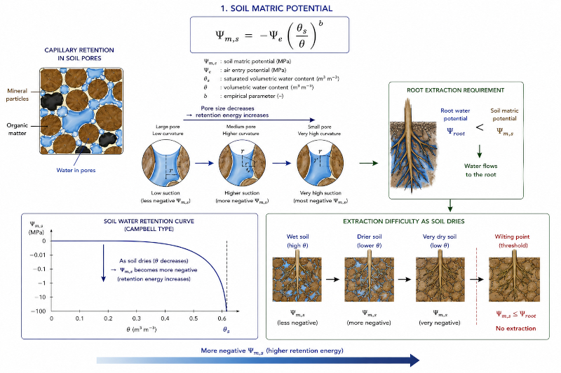
The image shows this process from the microscopic scale to its effect on the plant. In the upper left part you can see how water occupies the pores between the mineral particles and the organic matter. As the water content decreases, the capillary menisci become increasingly curved, increasing the energy needed to detach water from solid surfaces. This behavior is also represented by the water retention curve, where small decreases in water content cause increasingly pronounced decreases in matrix potential.
From the physiological point of view, this potential constitutes the initial condition for the entire water transport chain. The root can only absorb water when its own water potential is more negative than the matrix potential of the soil. As long as the soil remains moist, this condition is relatively easily satisfied and water flows to the root. However, as the soil dries, the required potential difference continually increases, making extraction difficult. Finally, the point of permanent wilting is reached, where the energy required to release the retained water exceeds the suction capacity of the root system and absorption practically stops.
Within the integrated model, this equation constitutes the mechanism that transforms the water content of the soil into an energy variable capable of driving or limiting all subsequent transport. The matrix potential determines how much energy the plant must invest to access the available water and therefore sets the boundary condition from which the flow into the xylem begins. Any change in soil moisture immediately modifies this potential and ends up propagating throughout the entire process chain, affecting hydraulic transport, the water status of the leaves, stomatal opening, photosynthesis and, finally, the efficiency with which the plant uses water.
ID:('gp', 629)
Soil osmotic $\Psi$
Storyboard
The equation describes the osmotic potential of the soil, that is, the decrease in the free energy of water caused by the presence of solutes dissolved in the solution that occupies the pores of the soil. Unlike the matrix potential, which arises from the capillary forces exerted by the solid matrix, the osmotic potential has its origin in the chemical composition of water. The higher the concentration of salts and other solutes, the lower the available energy of water and the more negative its osmotic potential becomes. This behavior corresponds directly to Van't Hoff's law for dilute solutions, which relates the osmotic potential to the solute concentration and absolute temperature.
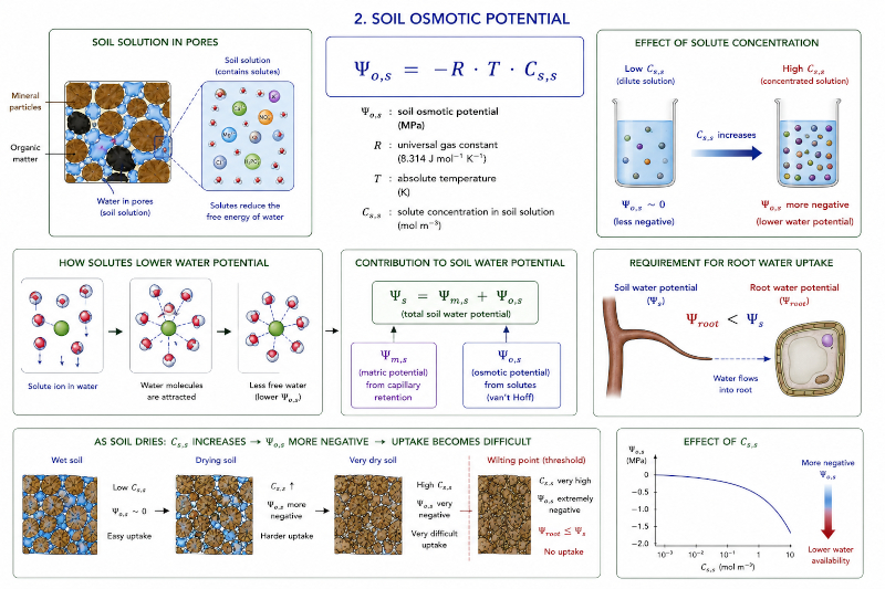
The image shows this mechanism from the microscopic scale to its consequences on root absorption. In the upper left part it is observed that the water present in the pores constitutes a solution that contains different dissolved ions. These particles attract and organize the water molecules around them, decreasing the fraction of free water capable of moving spontaneously. As a result, with increasing solute concentration the osmotic potential becomes progressively more negative, as illustrated by the sequence of dilute and concentrated solutions and the curve shown at the bottom right.
The osmotic potential does not act in isolation, but is one of the components that determine the total water potential of the soil. While the matrix potential represents the energy necessary to release water from mineral and organic surfaces, the osmotic potential represents the energy associated with the chemical composition of the soil solution. Both effects add up to establish the total energy with which water is available to the roots.
From a physiological point of view, an increase in the concentration of salts has an effect similar to drying out of the soil: although the water content may remain practically constant, the water becomes less energetically accessible to the plant. Consequently, the root must develop an even more negative water potential to maintain absorption. If this potential difference is no longer sufficient, the flow of water progressively decreases until it stops, generating a state of water stress even when water is physically present in the soil.
Within the integrated model, this equation incorporates the effect of soil chemical composition on water availability. Its function is to complement the physical effect of capillary retention, providing the second fundamental component of the soil's water potential. In this way, the model can represent both drought and salinity situations, both capable of reducing root absorption and propagating its effects throughout the entire process chain, modifying hydraulic transport, the water status of the leaves, stomatal regulation, photosynthesis and, finally, the efficiency with which the plant uses water.
ID:('gp', 630)
Soil water potential (total)
Storyboard
The equation defines the total water potential of the soil, which represents the effective energy with which water is available to be absorbed by the roots. Rather than relying on a single mechanism, this availability results from the combination of two different physical processes acting simultaneously. On the one hand, the capillary forces exerted by the matrix formed by mineral particles and organic matter retain water on the surfaces and within the pores of the soil. On the other hand, dissolved solutes decrease the free energy of water through osmotic effects. The total water potential summarizes both phenomena in a single variable that characterizes the energetic state of water in the soil.
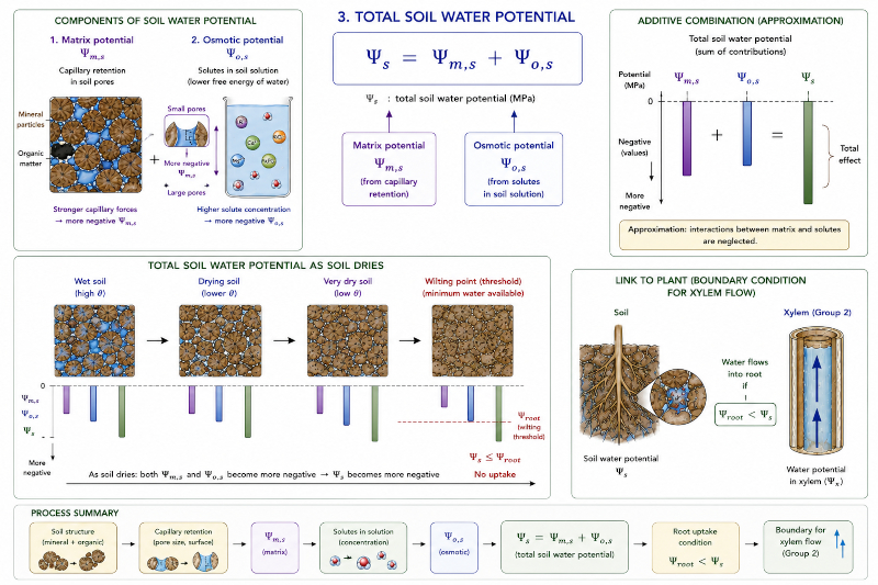
The image shows how these two mechanisms integrate to determine water availability. In the upper left part, the matrix potential, associated with capillary retention in the pores, and the osmotic potential, caused by the presence of solutes in the soil solution, are represented separately. Both contribute by making the water potential more negative. In the upper right part this combination is illustrated as a sum of energy contributions, highlighting that the total potential represents the joint effect of both processes, although the interaction between them is approximated by an additive superposition.
The central sequence shows how this potential evolves as the soil loses water. In a moist soil, both capillary retention and solute concentration exert a relatively moderate effect and the water potential remains high enough to allow root absorption. As the water content decreases, the intensity of capillary forces increases and simultaneously the concentration of solutes increases due to the reduction in the volume of available water. As a consequence, both components become progressively more negative and the total water potential continuously decreases. Finally, the wilting point is reached, where the soil potential becomes so negative that the root can no longer generate a sufficient gradient to extract water.
From the physiological point of view, the total water potential constitutes the initial condition that governs the entry of water to the plant. Absorption can only occur when the water potential of the root is more negative than that of the soil, so this variable directly determines whether the flow of water can be initiated and with what intensity it will do so. Any modification in the structure of the soil, in its water content or in the concentration of salts is immediately reflected in this potential and alters the water supply capacity of the entire plant.
Within the integrated model, this equation plays the role of closing the first group of processes. Its function is to bring together in a single variable the physical effects of capillary retention and the chemical effects of soil solution, providing the boundary condition that fuels hydraulic transport in the xylem. From this point, the complete chain of processes that connects the soil with the leaves begins, subsequently regulating water transport, foliar water status, stomatal opening, carbon fixation and, finally, the overall efficiency with which the plant uses water.
ID:('gp', 631)
Xylem flow (Darcy)
Storyboard
The equation describes the flow of water through the xylem, the conductive tissue responsible for transporting water from the roots to the leaves. This transport is driven by the difference in water potential between the soil and the leaf tissues. While the potential of the soil is relatively high and that of the leaves becomes more negative due to evaporation, an energy gradient is established that induces the continuous rise of the water column. The magnitude of the flow depends both on this potential difference and on the hydraulic capacity of the xylem to conduct water and the length of the path it must travel.
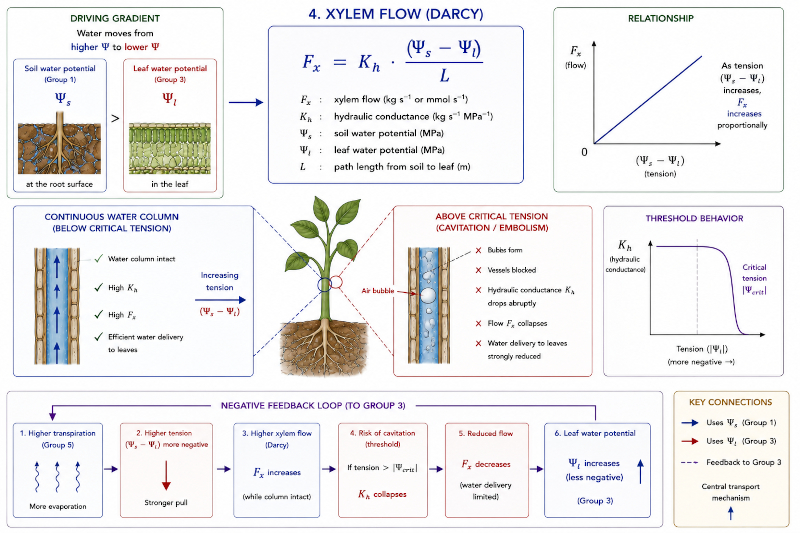
The image shows how this mechanism connects the soil with the atmosphere through a continuous column of water contained in the xylem vessels. The water absorbed by the roots rises driven by the tension generated in the leaves as a result of transpiration. This tension is transmitted throughout the entire column thanks to the cohesion between the water molecules and their adhesion to the walls of the conductive vessels, allowing water to be extracted from the ground even to great heights. As long as the continuity of the column is maintained, transport is highly efficient and responds approximately proportionally to the water potential gradient.
However, this mechanism has a physical limit. When the voltage increases excessively, air bubbles can form inside the conductive vessels. This phenomenon, known as cavitation or embolism, disrupts the continuity of the water column and reduces the xylem's ability to transport water. Consequently, although the potential gradient continues to increase, the flux can no longer increase in the same proportion because part of the conductive network is no longer functional. The plant then enters a regime where hydraulic transport is limited by the deterioration of the conductive system itself.
From a physiological point of view, xylem flow constitutes the link that connects soil conditions with the water status of the leaves. The amount of water that reaches the leaf tissues depends directly on this transport and determines the ability to maintain cell turgor, sustain transpiration and allow the opening of the stomata. At the same time, the water potential of the leaves influences the gradient that drives flow, establishing a continuous feedback between water supply and leaf water status.
Within the integrated model, this equation represents the central physical mechanism of water transport in the plant. It receives as an initial condition the total water potential of the soil calculated in the previous group and uses as a final condition the water potential of the leaf, which will be determined later by the balance between water entry and loss. In this way, xylem flow constitutes the link between the availability of water in the soil and the physiological regulation that occurs in the leaves. Any decrease in the hydraulic capacity of the xylem, whether due to cavitation or other limitations, reduces the supply of water to the leaf tissues and triggers a cascade of responses that affect stomatal aperture, photosynthesis, transpiration and, finally, the overall efficiency with which the plant uses water.
ID:('gp', 632)
Vulnerability curve
Storyboard
The equation describes the vulnerability of the plant's hydraulic system to cavitation, that is, the progressive loss of water conduction capacity as tension in the xylem increases. While the water rises driven by evaporation from the leaves, the liquid column remains stable thanks to the cohesive forces between the water molecules. However, when the xylem water potential reaches sufficiently negative values, the tension exceeds a critical threshold and air bubbles begin to form within the conductive vessels. These bubbles disrupt the continuity of the water column and reduce the number of conduits that remain operational for transport.
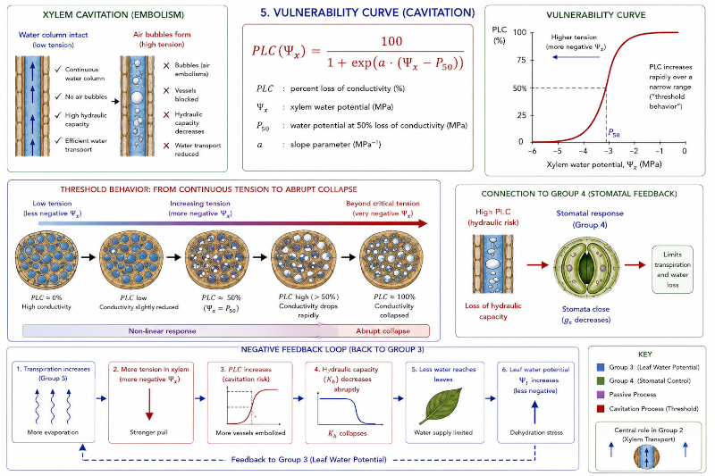
The image shows this process as a transition between a fully functional hydraulic system and one progressively clogged by embolisms. In a low-tension state, virtually all vessels remain full of water and the hydraulic capacity is maximum. As the stress increases, isolated cavitations begin to appear, slowly reducing the effective surface area available for transport. Finally, a critical region is reached where a small additional decrease in water potential causes rapid propagation of embolisms and an abrupt loss of conductivity. This behavior is represented by a sigmoidal curve, characteristic of a phenomenon governed by a physical threshold rather than a linear decrease.
One of the most important parameters of this relationship is the potential for which the plant has lost approximately half of its conducting capacity. This value constitutes a measure of xylem resistance to cavitation and varies between species depending on their adaptation to humid or dry environments. Plants adapted to arid conditions usually tolerate much more negative potentials before experiencing significant losses in conductivity, while species from humid environments present less extreme thresholds.
From a physiological point of view, cavitation represents a protection mechanism and, at the same time, a limitation for the functioning of the plant. The loss of conductivity reduces the supply of water to the leaves, decreasing leaf water potential and increasing water stress. As a consequence, the plant responds by progressively closing the stomata to reduce transpiration and prevent tension from continuing to increase. In this way, a negative feedback mechanism is established that seeks to prevent irreversible hydraulic collapse.
Within the integrated model, this equation constitutes the nonlinear trigger of hydraulic transport. While the xylem flow equation describes an approximately proportional behavior between the potential gradient and water transport, this relationship introduces the physical limit of the system by transforming a continuous increase in tension into a sudden loss of conductive capacity. The vulnerability obtained directly feeds the calculation of the effective hydraulic capacity of the xylem and, subsequently, stomatal regulation. Thanks to this mechanism, the model can represent one of the most important phenomena in plant physiology: the existence of a functioning threshold beyond which the hydraulic system gradually stops responding and enters a regime of accelerated deterioration that conditions the entire balance between water transport, photosynthesis and plant survival.
ID:('gp', 633)
Effective hydraulic capacity
Storyboard
The equation describes the effective hydraulic capacity of the xylem, that is, the fraction of the maximum water transport capacity that remains available after part of the conducting vessels has been rendered useless by cavitation. While the maximum hydraulic capacity represents the ideal functioning of a vascular network completely filled with water, the effective capacity reflects the real state of the system under the existing stress conditions. As the number of vessels blocked by embolism increases, the surface area available to conduct water decreases and, consequently, hydraulic transport is reduced in the same proportion.
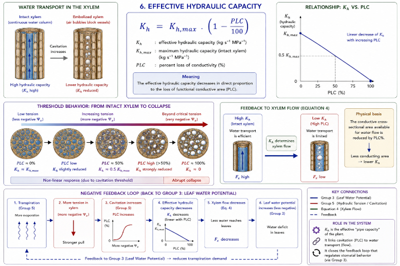
The image shows how the vascular system evolves from a fully functional state to one where an increasing fraction of the vessels stop participating in transport. Initially, the entire conductive network is available and water can rise without significant restrictions. As cavitations appear, some ducts become filled with air and stop transmitting the tension generated by foliar evaporation. Water must then circulate through an increasingly smaller number of active vessels, reducing the overall transport capacity. When the loss of conductivity reaches high values, the system enters a regime where even large differences in water potential are unable to maintain sufficient flow to the leaves.
From the physical point of view, this relationship constitutes the natural closure of the cavitation process. The previous equation determines what fraction of the vascular network has stopped functioning as a consequence of the formation of embolisms, while this equation directly transforms this structural loss into a decrease in hydraulic conductivity. In this way, the model connects the microscopic state of the xylem with its macroscopic behavior as a transport system, maintaining coherence between the effective geometry of the ducts and the flow they can sustain.
The physiological consequences are immediate. A lower hydraulic capacity implies that less water reaches the leaves for the same water potential gradient. As a result, tissue hydration decreases, leaf water potential becomes more negative and water stress increases. Faced with this situation, the plant responds by reducing the stomatal opening to reduce transpiration and prevent the tension in the xylem from continuing to increase. This response constitutes a protection mechanism that attempts to stabilize the system before the loss of conductivity reaches irreversible levels.
Within the integrated model, this equation represents the closure of the group dedicated to hydraulic transportation. Its function is to continually update the true capacity of the xylem from the previously calculated cavitation level and use this new value to determine the flow of water to the leaves. A feedback loop is thus established where the increase in tension favors cavitation, cavitation reduces the hydraulic capacity and this reduction decreases the upward flow of water. As a consequence, the effective hydraulic capacity becomes one of the variables that directly connect the structural state of the vascular system with the physiological regulation of the plant, propagating its effects towards the foliar water state, stomatal opening, photosynthesis and global efficiency in water use.
ID:('gp', 634)
Leaf water balance (dynamic)
Storyboard
The equation describes the dynamic balance of water in the leaf, simultaneously considering the water that enters from the xylem and the water that is lost through transpiration to the atmosphere. Unlike the previous equations, which represent instantaneous relationships between variables, this one explicitly incorporates the temporal evolution of the system. The hydric state of the leaf no longer depends only on the present conditions, but also on the recent history of water transport and the losses that have occurred due to evaporation. The leaf thus acts as a small reservoir whose hydration increases when the supply exceeds the losses and decreases when the opposite situation occurs.
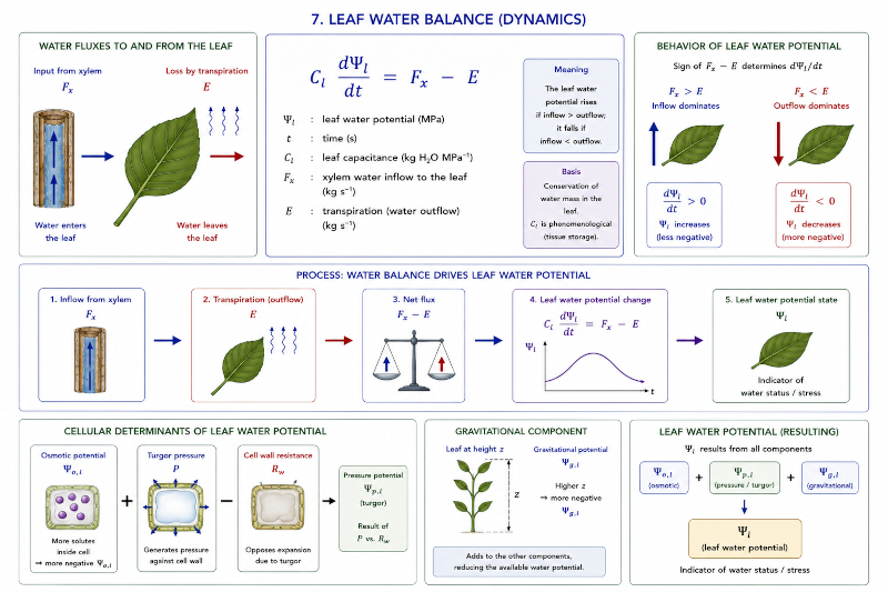
The image shows this balance as the point where two opposite flows converge. From the bottom comes the water transported by the xylem, while from the leaf surface the water continually leaves the plant through transpiration. As long as both flows remain balanced, the leaf water content remains approximately constant and the water potential remains stable. If transport from the roots increases or transpiration decreases, the leaf recovers water and its water potential becomes less negative. On the other hand, when evaporation exceeds the supply from the xylem, the leaf loses water, its water content decreases and the potential becomes progressively more negative, indicating an increase in water stress.
The presence of a water capacitance reflects that leaf tissues have the capacity to temporarily store water. This storage buffers rapid variations in the environment, preventing small instantaneous changes in solar radiation, atmospheric humidity or stomatal opening from producing equally abrupt changes in the plant's water status. Thanks to this inertia, the system responds continuously and stably, reproducing the behavior observed experimentally in plant tissues.
From a physiological point of view, foliar water potential constitutes one of the most important indicators of the state of the plant. When the water supply is sufficient, cells maintain their hydration, maintain turgor, and can sustain high physiological activity. On the contrary, when losses persistently exceed supply, water potential decreases, water stress increases and regulatory mechanisms designed to conserve water begin to activate, especially the progressive closure of the stomata.
Within the integrated model, this equation constitutes the dynamic core of the water state of the leaf. It receives the water flow calculated by the hydraulic model of the xylem and confronts it with the water loss determined by transpiration. The resulting water potential not only describes the instantaneous physiological condition of the leaf tissues, but also feeds back to hydraulic transport by modifying the potential gradient that drives the rise of water from the roots. In this way, the water status of the leaf becomes the meeting point between the availability of water in the soil, vascular transport and stomatal regulation, integrating into a single variable the dynamic response of the entire plant to changing environmental conditions.
ID:('gp', 635)
Decomposition of leaf potential
Storyboard
The equation decomposes the water potential of the leaf into its main physical components, allowing us to understand what mechanisms determine the energetic state of water within the leaf tissues. Instead of considering water potential as a single global variable, this relationship shows that the behavior of the leaf results from the balance between the pressure exerted by water on the cell walls, the effect of the solutes present inside the cells and the difference in energy associated with the position of the leaf within the gravitational field. In this way, water potential stops being a simple indicator of hydration and begins to be interpreted as the consequence of several physical processes that act simultaneously.
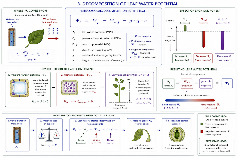
The image illustrates how each of these components contributes to the water status of the leaf. Turgor pressure represents the mechanical effect produced when the cell vacuole fills with water and pushes the membrane against the cell wall, providing rigidity to the tissues. The osmotic potential acts in the opposite direction, caused by the presence of solutes inside the cells, which reduce the free energy of water and favor its entry from less concentrated regions. Added to these two mechanisms is the gravitational effect, which reflects the energy necessary to maintain the water at a certain height within the plant. Although the latter is usually small in short plants, it becomes important in large trees, where crown elevation represents an appreciable fraction of the water potential gradient.
Each of these components responds to different physiological processes. Turgor depends on the water content of the cells and determines the rigidity of leaves and stems, directly influencing the growth and normal functioning of tissues. Osmotic potential is governed by cellular solute concentration, which can be modified by osmotic adjustments that help the plant tolerate drought or salinity conditions. The gravitational component, on the other hand, depends exclusively on height and constitutes a permanent physical restriction that must be compensated by the hydraulic system during water transport.
From a physiological point of view, this decomposition allows us to interpret the origin of the water stress observed in a leaf. The same value of water potential can be due to a loss of turgor caused by dehydration, an increase in the concentration of solutes as an adaptation mechanism, or simply to the elevated position of the leaf within the plant. Therefore, the equation provides a tool to distinguish between different physiological states that, although they present a similar water potential, have very different causes and consequences.
Within the integrated model, this equation does not introduce a new dynamic mechanism, but rather fulfills a diagnostic function. The dynamic water balance determines how the leaf's water potential evolves over time, while this relationship explains how said potential is distributed among its fundamental physical components. Thanks to this decomposition, the model can directly relate hydraulic transport, cellular hydration, osmotic regulation and the effects of gravity, providing a physical interpretation of the leaf water state that will subsequently influence stomatal opening, transpiration and photosynthetic activity.
ID:('gp', 636)
Leaf osmotic potential
Storyboard
The equation describes the osmotic potential of the interior of the leaf, that is, the contribution made by the concentration of solutes present in the cells to the energy state of the water. Inside the leaf tissue, water is not found in its pure state, but forming a solution that contains sugars, salts, amino acids and numerous compounds produced by cellular metabolism. The presence of these substances reduces the free energy of water, making the osmotic potential always negative. The higher the concentration of solutes, the more negative this potential becomes and the greater the tendency for water to move into the cells.
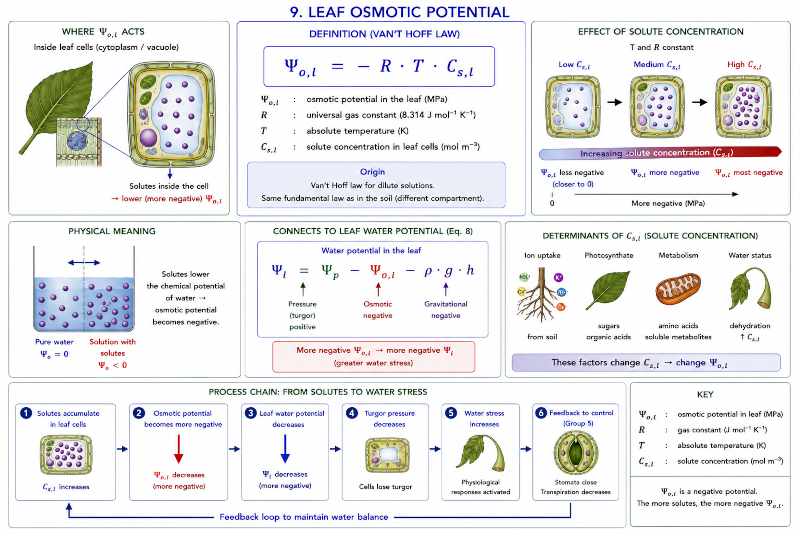
The image shows this process from the cellular scale to its effect on leaf function. Inside the mesophyll cells, the vacuole accumulates a high concentration of solutes, while water from the xylem enters following the water potential gradient. As the concentration of solutes increases, water molecules become more strongly associated with them, decreasing their free energy. This behavior corresponds directly to Van't Hoff's law for dilute solutions and constitutes the same physical principle previously used to describe the osmotic potential of the soil, although now applied to the cellular compartment of the leaf.
From a physiological point of view, osmotic potential plays an essential role in maintaining cellular hydration. The accumulation of solutes allows water to be attracted into the cells even when the external water potential decreases as a result of drought. Many species use this mechanism as an adaptive strategy, synthesizing or accumulating osmotically active compounds that reduce osmotic potential without interfering with metabolism. Thanks to this osmotic adjustment, cells can conserve their water content and maintain turgor even under conditions of water stress.
The osmotic potential also directly influences the turgor pressure. When water enters the cells driven by the osmotic gradient, the vacuole expands and exerts pressure on the cell wall, providing rigidity to the tissues and allowing the leaf to retain its structure. If the osmotic potential stops compensating for water losses through transpiration, water intake decreases, turgor falls and the leaf begins to lose rigidity, appearing the first signs of wilting.
Within the integrated model, this equation provides one of the fundamental components of foliar water potential. The dynamic water balance determines how the water content of the leaf evolves, while the decomposition of the water potential uses the osmotic potential to explain an essential part of that energy. In this way, the concentration of solutes establishes a link between internal biochemical processes and the hydraulic behavior of the plant. Modifications of the osmotic potential alter the water status of the cells, affect turgor and end up influencing stomatal regulation, transpiration, photosynthesis and the plant's ability to withstand periods of water deficit.
ID:('gp', 637)
Höfler ratio (turgor)
Storyboard
The equation describes how turgor pressure is generated inside plant cells as a consequence of the entry of water. When water enters the vacuole driven by the water potential gradient, cell volume increases and the plasma membrane presses against the cell wall. As this wall has considerable mechanical resistance, it opposes expansion and develops an internal pressure that keeps the tissues rigid. The relationship establishes that this pressure appears only when the cell volume exceeds a reference volume. As long as the cell remains below this threshold, the wall is not yet compressed and the turgor pressure is practically zero. Once this point is exceeded, the pressure increases approximately proportional to the degree of expansion of the cell.
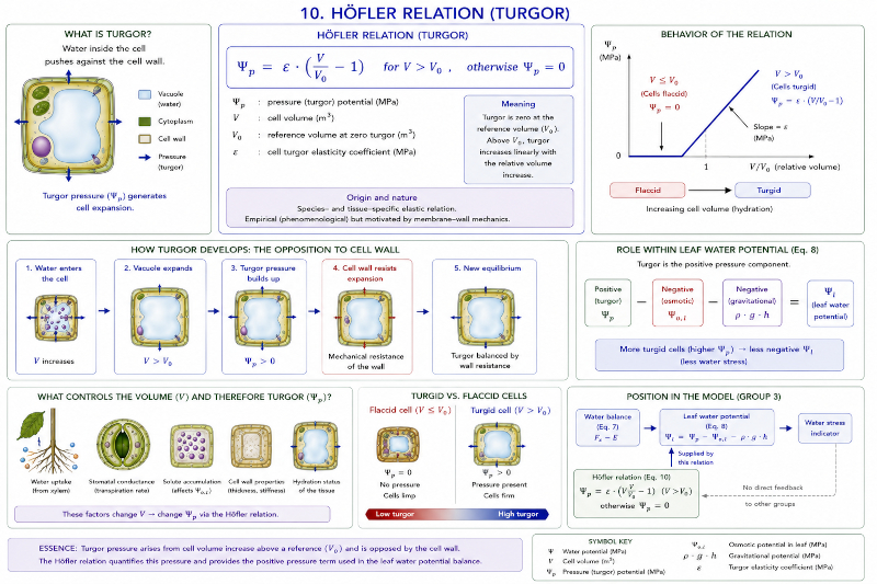
The image shows this process through a sequence of cells with different hydration states. In a well-hydrated cell, the vacuole occupies much of the internal volume and exerts uniform pressure on the cell wall, keeping the tissue firm and the leaf extended. When the availability of water decreases, the vacuole loses volume, the internal pressure drops and the wall is no longer completely stressed. If the loss of water continues, the cell enters a flaccid state where turgor pressure practically disappears and the tissues begin to lose rigidity, manifesting the characteristic wilting of a plant subjected to water stress.
From the physical point of view, turgor pressure constitutes the mechanical component of foliar water potential. While the osmotic potential favors the entry of water into the cell, the elasticity of the cell wall generates an opposing force that limits expansion. The balance between both effects determines the mechanical state of the tissues. The elastic parameter used in the relationship precisely represents the stiffness of the cell wall and expresses how much the internal pressure increases when the cell volume is increased above its reference state. Different species have different values of this parameter, reflecting structural adaptations to their environmental conditions.
From a physiological point of view, turgor is essential for the normal functioning of the plant. The rigidity of leaves, young stems and growing organs depends directly on this internal pressure. Furthermore, numerous physiological processes, such as cell expansion, tissue growth, and the movement of certain plant organs, require maintaining adequate turgor pressure. When this decreases as a result of water loss, the plant not only reduces its growth capacity, but also increases its vulnerability to environmental stress.
Within the integrated model, this equation completes the physical description of leaf water potential by providing the pressure component necessary to interpret the hydration state of the cells. The dynamic water balance determines how much water the leaf contains, the osmotic potential explains the effect of solutes on that water, and the Höfler relation transforms that water content into an observable mechanical response. Although this pressure does not act directly on other groups in the model, it constitutes a fundamental indicator of the physiological state of the tissues and allows us to interpret how variations in hydraulic transport and transpiration end up affecting the mechanical stability, growth and functional capacity of the plant.
ID:('gp', 638)
Base stomatal conductance (Ball-Berry)
Storyboard
The equation describes the basal stomatal conductance, that is, the degree of opening that the stomata would have considering only the physiological signals associated with photosynthesis, the relative humidity on the leaf surface and the availability of carbon dioxide. Stomata constitute the main mechanism for regulating gas exchange between the plant and the atmosphere. Through them, the carbon dioxide necessary for photosynthesis enters, but simultaneously water is lost in the form of vapor. Therefore, stomatal opening represents a permanent compromise between two opposing processes: maximizing carbon capture and minimizing water loss.
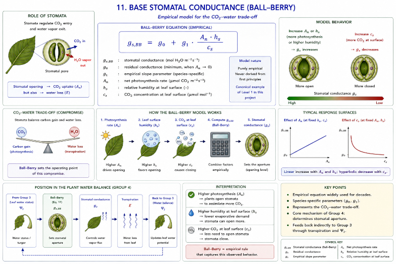
The image shows this balance by representing a stoma whose opening simultaneously controls the entry of CO and the exit of water vapor. When photosynthetic activity increases, the demand for carbon dioxide also increases and the stomatal opening tends to be larger to facilitate its diffusion into the leaf. Similarly, a more humid atmosphere reduces the water cost associated with keeping stomata open, also favoring greater conductance. On the other hand, a high concentration of carbon dioxide on the leaf surface reduces the need to open the stomata widely, since the gas can enter more easily even when the opening is smaller. The combination of these factors determines a basal level of opening that represents the expected performance of the system before considering other hydraulic limitations.
From the physiological point of view, this relationship summarizes the behavior observed experimentally in numerous plant species. It is not intended to describe the biochemical or cellular mechanisms responsible for the movement of occlusive cells, but rather to reproduce the global result of these processes through an empirical expression adjusted to observations. Therefore, it constitutes a description of the average behavior of the stomata under normal operating conditions, where the plant does not yet experience severe restrictions on water availability.
The most important concept introduced by this equation is that stomatal opening depends simultaneously on the photosynthetic state and atmospheric conditions. Stomata do not respond exclusively to water deficit or solely to the availability of carbon dioxide, but rather integrate multiple signals to select an operating point that allows maintaining efficient gas exchange without unnecessarily increasing water consumption. This integration makes the stomata the main control point of the entire physiological system.
Within the integrated model, this equation represents the central regulatory mechanism that connects hydraulic processes with photosynthetic processes. From this baseline value, the actual stomatal opening will subsequently be determined, once the effect of cavitation and hydraulic stress has been incorporated. In this way, the basal conductance constitutes the reference point on which the system's feedbacks act. The resulting opening will simultaneously control transpiration and the influx of carbon dioxide, establishing the link between the plant's water status and its ability to fix carbon. For this reason, stomatal conductance becomes the control variable shared by practically all the processes of the model and the origin of the structural compromise that prevents simultaneous optimization of water conservation and photosynthetic productivity.
ID:('gp', 639)
Final Conductance (with hydraulic feedback)
Storyboard
The equation describes the effective stomatal conductance, that is, the actual opening of the stomata once the plant incorporates the state of its hydraulic system. While the basal conductance represents the level of aperture expected from the photosynthetic and atmospheric conditions, the effective aperture incorporates an additional mechanism of protection against the risk of cavitation. In this way, the plant does not regulate the stomata only to optimize the exchange of carbon dioxide and water vapor, but also to prevent hydraulic transport from reaching stress levels capable of causing irreversible damage to the xylem.
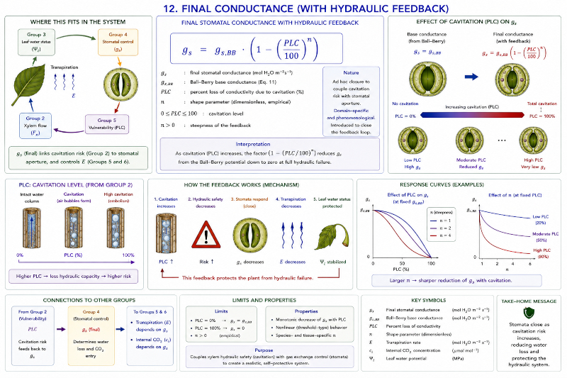
The image shows how the state of the vascular system progressively modifies the stomatal opening. When the xylem retains practically all of its conductive capacity, the hydraulic risk is very low and the effective conductance almost coincides with the basal conductance. Under these conditions the stomata remain relatively open, favoring both the entry of carbon dioxide and the exit of water vapor. However, as cavitation increases and an increasing fraction of the conductive vessels cease to function, the plant begins to deliberately reduce the stomatal aperture. This response limits transpiration, reduces tension in the water column and reduces the probability of new embolisms appearing.
From a physiological point of view, this mechanism constitutes a preventive response to water stress. The plant does not wait for the hydraulic system to completely collapse, but rather uses the degree of conductivity loss as a signal to continually adjust the opening of the stomata. When the hydraulic damage is still small, the regulation barely modifies the gas exchange. On the other hand, as the vulnerability threshold is approached, small additional losses of conductivity produce increasingly important reductions in stomatal aperture. As a consequence, the system presents a strongly non-linear response that allows the water transport to be protected before reaching a critical state.
This behavior introduces one of the main negative feedback mechanisms of the model. An increase in transpiration increases tension in the xylem, favoring cavitation. Cavitation reduces the hydraulic capacity and, through this equation, induces the progressive closure of the stomata. By decreasing the stomatal opening, the loss of water through evaporation also decreases, again reducing the tension on the vascular system. Thanks to this regulation cycle, the plant manages to stabilize its operation in the face of environmental changes such as increases in temperature, decreases in atmospheric humidity or reductions in the availability of soil water.
Within the integrated model, this equation constitutes the coupling point between hydraulics and gas exchange. It is the mechanism by which the state of the xylem directly modifies stomatal regulation, connecting water transport with photosynthesis and transpiration. The resulting conductance simultaneously feeds the water loss and carbon dioxide diffusion models, becoming the control variable shared by both processes. Thanks to this feedback, the model reproduces the fundamental physiological commitment of plants: maintaining sufficient opening to sustain carbon fixation, but closing it opportunely when the risk of cavitation threatens the continuity of the hydraulic system.
ID:('gp', 640)
Perspiration (vapor diffusion)
Storyboard
The equation describes the transpiration rate, that is, the speed with which water leaves the plant in the form of vapor through the stomata. This process constitutes the main mechanism of water loss in the plant, but at the same time it is the physical engine that maintains hydraulic transport from the roots to the leaves. Continuous evaporation on the leaf surface generates tension in the water column contained in the xylem, which is transmitted downwards thanks to the cohesion between water molecules, allowing new amounts of water to be extracted from the soil.
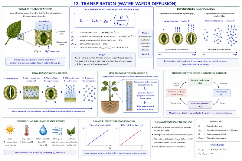
The image shows how perspiration arises from the interaction between two fundamental factors. The first is the stomatal opening, which determines the size of the path available for water vapor diffusion. The larger the opening of the stomata, the lower the resistance to the passage of vapor and the greater the water loss. The second is the humidity deficit between the interior of the leaf and the atmosphere. As the outside air remains relatively dry, the vapor concentration difference increases and the diffusive flow intensifies. Both factors act together: a wide opening only produces high transpiration if there is also a strong humidity gradient, while very dry air barely causes significant losses when the stomata remain closed.
From the physical point of view, the equation corresponds to an adaptation of Fick's diffusion law for the transport of water vapor. The diffusion speed is proportional to both the stomatal conductance and the driving force generated by the vapor gradient. The constant factor incorporated in the expression does not represent an empirical adjustment, but rather the difference between the diffusive properties of water vapor and carbon dioxide in the air. Thanks to this, the equation maintains a direct connection with the fundamental laws of molecular transport.
The physiological consequences of this process are profound. Greater transpiration increases the water supply and favors the cooling of the leaves, but it also increases the plant's water consumption and the tension supported by the vascular system. When atmospheric conditions are very dry or the stomata remain excessively open, the flow of water can exceed the capacity of the xylem to supply the tissues, favoring the development of cavitation and increasing the risk of water stress. On the contrary, an excessive reduction in transpiration protects the hydraulic system, although it simultaneously limits the gas exchange necessary for photosynthesis.
Within the integrated model, this equation constitutes the mechanism that transforms stomatal regulation and atmospheric conditions into a real water outflow. The stomatal conductance calculated in the previous group determines how much the vapor can diffuse, while the environment sets the intensity of the driving force. The resulting flow directly feeds the water balance of the leaf and, at the same time, generates the tension that drives the rise of water through the xylem. In this way, transpiration establishes the link between the physiological regulation of the stomata and the hydraulic transport of the entire plant, becoming one of the central processes that connect water availability, gas exchange and survival against water stress.
ID:('gp', 641)
Steady State Closure
Storyboard
The equation expresses one of the fundamental conditions for the stable operation of the plant's water transport system. In a quasi-steady state, the amount of water rising from the roots through the xylem must be equal to the amount of water leaving the plant through transpiration. In other words, the water that continually reaches the leaves is exactly what is needed to replace that which evaporates into the atmosphere, so that the water content stored in the tissues remains practically constant. This relationship constitutes a direct consequence of the principle of mass conservation applied to the soil-plant-atmosphere continuum.
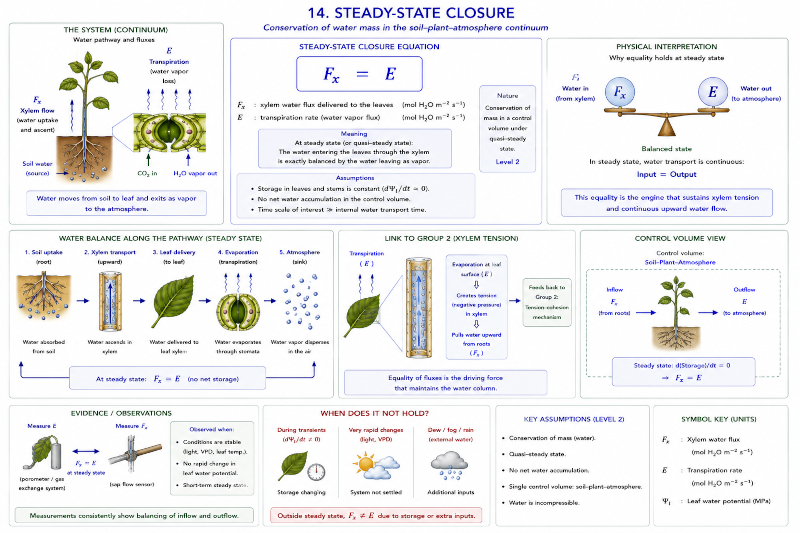
The image shows this balance as a continuous flow that connects the ground with the atmosphere. The water absorbed by the roots ascends through the xylem driven by the tension generated in the leaves and, finally, evaporates through the stomata. As long as the system remains in equilibrium, there is no accumulation or net loss of water within the plant. Each molecule that leaves the leaf is replaced by another that ascends from the root system, keeping the water state of the tissues stable. The plant thus behaves as a dynamic conduit through which water continuously circulates from the soil to the atmosphere.
From the physical point of view, this equality represents the natural closure of the mass balance of water. It does not introduce a new transport mechanism, but rather establishes the condition that xylem hydraulic flow and water loss through evaporation must be satisfied simultaneously when the system operates stably. If, due to some environmental disturbance, transpiration increases faster than the upward flow, the leaf begins to lose water, the leaf water potential decreases and the system momentarily leaves equilibrium. Similarly, if the water supply temporarily exceeds evaporation, the leaf recovers water and the water potential increases until it reaches a state of balance again.
This balance explains why transpiration is the true engine of hydraulic transport. Evaporation represents not only a loss of water, but the physical process that generates the stress necessary to continually extract water from the ground.
The greater the evaporation, the greater the hydraulic demand that the xylem must satisfy. As long as the vascular system retains sufficient conductive capacity, ascending flow increases to compensate for this demand. However, when the hydraulic capacity decreases due to cavitation, the flow can no longer follow the increase in transpiration and the balance begins to break, triggering a decrease in leaf water potential and the activation of stomatal closure.
Within the integrated model, this equation constitutes the closure of the group dedicated to transpiration and the point where the feedback loop between evaporation and hydraulic transport is completed. The flow calculated by the xylem model feeds the water balance of the leaf, while transpiration generates the tension that drives that same flow again. A closed circuit is thus formed that connects the soil, the vascular system, the leaves and the atmosphere through a single continuous process of mass conservation. Thanks to this relationship, the model explicitly represents that water transport and transpiration are not independent processes, but rather two complementary manifestations of the same hydraulic flow that maintains the operation of the entire plant.
ID:('gp', 642)
CO2 supply (diffusion)
Storyboard
The equation describes the supply of carbon dioxide to the interior of the leaf, that is, the speed with which atmospheric $CO_2$ enters through the stomata and diffuses to the intercellular spaces where it will later be used by photosynthesis. This process constitutes the carbon supply stage and depends simultaneously on two factors. On the one hand, the stomatal opening determines the size of the path available for gas diffusion. On the other hand, the difference between the concentration of $CO_2$ in the air and that existing inside the leaf provides the driving force that moves the molecules towards the mesophyll. The larger the stomatal opening and the greater the concentration gradient, the more intense the influx of carbon dioxide will be.
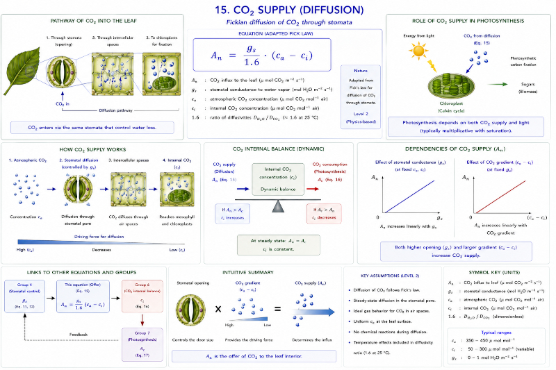
The image shows this journey from the atmosphere to the chloroplasts. Carbon dioxide first passes through the open stomata, diffuses through the intercellular spaces and finally reaches the photosynthetic cells. During this journey, the concentration of the gas progressively decreases because the molecules are consumed by photosynthesis. As long as there is a difference between the atmospheric concentration and the internal concentration, diffusion continues to feed the system. If photosynthetic activity increases and consumes $CO_2$ more quickly, the internal concentration decreases, increasing the gradient and favoring greater gas entry. On the other hand, when the stomata close or the gradient is reduced, the carbon supply immediately decreases.
From the physical point of view, this relationship corresponds to an application of Fick's law for molecular diffusion. The flux of carbon dioxide is proportional to both the stomatal conductance and the concentration gradient between the outside and inside of the leaf. The constant factor present in the expression is not an experimentally adjusted parameter, but rather reflects the difference between the diffusive properties of carbon dioxide and water vapor in the air. Thanks to this, the equation maintains a direct connection with the fundamental laws of diffusion transport and, at the same time, maintains coherence with the transpiration model used previously.
From the physiological point of view, this equation reveals the central commitment of plant physiology. The same stomata that allow carbon dioxide to enter are also the main route of water loss through transpiration. Opening the stomata favors the supply of carbon necessary for photosynthesis, but simultaneously increases evaporation and the risk of cavitation of the hydraulic system. Reducing the aperture protects water transport, although it immediately limits the availability of $CO_2$ to chloroplasts. This competition between carbon acquisition and water conservation constitutes one of the fundamental principles of plant operation.
Within the integrated model, this equation represents the supply side of the carbon dioxide balance. Stomatal regulation determines the supply capacity, while photosynthetic consumption, described later, constitutes the system demand. The balance between both processes establishes the internal concentration of $CO_2$ and, with it, the amount of carbon available for photosynthesis. In this way, the diffusion of carbon dioxide directly connects the plant's hydraulics with its photosynthetic metabolism, integrating stomatal regulation, gas exchange and biomass production into a single process that will ultimately determine the efficiency of water use.
ID:('gp', 643)
Photosynthetic demand (light-limited Michaelis-Menten)
Storyboard
The equation describes the supply of carbon dioxide to the interior of the leaf, that is, the speed with which atmospheric $CO_2$ enters through the stomata and diffuses to the intercellular spaces where it will later be used by photosynthesis. This process constitutes the carbon supply stage and depends simultaneously on two factors. On the one hand, the stomatal opening determines the size of the path available for gas diffusion. On the other hand, the difference between the concentration of $CO_2$ in the air and that existing inside the leaf provides the driving force that moves the molecules towards the mesophyll. The larger the stomatal opening and the greater the concentration gradient, the more intense the influx of carbon dioxide will be.
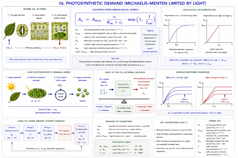
The image shows this journey from the atmosphere to the chloroplasts. Carbon dioxide first passes through the open stomata, diffuses through the intercellular spaces and finally reaches the photosynthetic cells. During this journey, the concentration of the gas progressively decreases because the molecules are consumed by photosynthesis. As long as there is a difference between the atmospheric concentration and the internal concentration, diffusion continues to feed the system. If photosynthetic activity increases and consumes $CO_2$ more quickly, the internal concentration decreases, increasing the gradient and favoring greater gas entry. On the other hand, when the stomata close or the gradient is reduced, the carbon supply immediately decreases.
From the physical point of view, this relationship corresponds to an application of Fick's law for molecular diffusion. The flux of carbon dioxide is proportional to both the stomatal conductance and the concentration gradient between the outside and inside of the leaf. The constant factor present in the expression is not an experimentally adjusted parameter, but rather reflects the difference between the diffusive properties of carbon dioxide and water vapor in the air. Thanks to this, the equation maintains a direct connection with the fundamental laws of diffusion transport and, at the same time, maintains coherence with the transpiration model used previously.
From the physiological point of view, this equation reveals the central commitment of plant physiology. The same stomata that allow carbon dioxide to enter are also the main route of water loss through transpiration. Opening the stomata favors the supply of carbon necessary for photosynthesis, but simultaneously increases evaporation and the risk of cavitation of the hydraulic system. Reducing the aperture protects water transport, although it immediately limits the availability of $CO_2$ to chloroplasts. This competition between carbon acquisition and water conservation constitutes one of the fundamental principles of plant operation.
Within the integrated model, this equation represents the supply side of the carbon dioxide balance. Stomatal regulation determines the supply capacity, while photosynthetic consumption, described later, constitutes the system demand. The balance between both processes establishes the internal concentration of $CO_2$ and, with it, the amount of carbon available for photosynthesis. In this way, the diffusion of carbon dioxide directly connects the plant's hydraulics with its photosynthetic metabolism, integrating stomatal regulation, gas exchange and biomass production into a single process that will ultimately determine the efficiency of water use.
ID:('gp', 644)
Dynamic internal $CO_2$ balance
Storyboard
The equation describes how the internal concentration of carbon dioxide within the leaf evolves over time as a result of the balance between two opposite processes: the entry of $CO_2$ from the atmosphere and its consumption by photosynthesis. Unlike the two previous equations, which represent carbon supply and demand separately, this one integrates both processes into a single dynamic balance. The internal concentration does not remain fixed, but changes continuously depending on which of the two processes predominates at each moment. When supply exceeds consumption, concentration increases; When photosynthesis consumes carbon faster than it can take in, the concentration decreases until a new equilibrium state is reached.
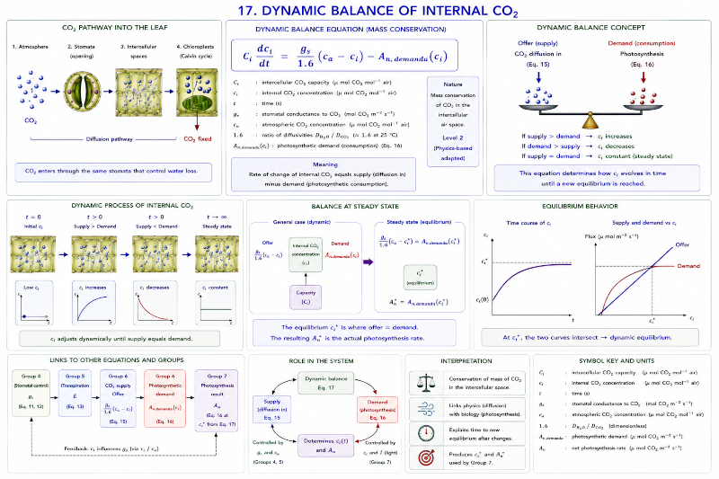
The image shows this balance as a system of inputs and outputs centered on the intercellular spaces of the leaf. Carbon dioxide diffuses from the atmosphere through the stomata and feeds a reservoir represented by the internal concentration. From that same reservoir, carbon is continuously extracted by chloroplasts to be incorporated into organic compounds through photosynthesis. As long as both velocities are equal, the concentration remains stable. If the stomatal aperture increases or the atmospheric concentration is high, the supply of $CO_2$ increases and the internal concentration tends to increase. On the contrary, if radiation increases and accelerates photosynthesis without an equivalent increase in supply, the internal concentration decreases until both processes compensate again.
From the physical point of view, this equation constitutes a direct application of the principle of conservation of mass to the carbon dioxide contained in the intercellular spaces of the leaf. The temporal change in the amount of $CO_2$ stored is equal to the difference between the flow that enters and the flow that is consumed. The presence of a capacitance for carbon dioxide represents the capacity of the intercellular volume to temporarily store the gas, preventing small instantaneous variations in stomatal opening or light intensity from producing abrupt changes in the internal concentration. Thanks to this inertia, the system responds continuously and reproduces the behavior observed experimentally during transitions between different environmental conditions.
From the physiological point of view, the internal concentration of $CO_2$ constitutes one of the key variables that regulate photosynthetic activity. If it decreases excessively, carbon fixation begins to be limited by the availability of the gas, even when there is abundant light. If it increases too much, photosynthesis stops benefiting from further increases due to saturation of the biochemical machinery. The system naturally tends toward an operating point where carbon supply through the stomata and photosynthetic consumption remain balanced, continually adjusting the internal concentration in the face of changes in radiation, atmospheric humidity, or water availability.
Within the integrated model, this equation constitutes the dynamic closure of the carbon dioxide exchange. It receives the inflow calculated by the diffusion model and the outflow determined by the photosynthetic demand, generating the internal concentration that feeds the carbon fixation process again. A feedback loop is thus established between diffusion and photosynthesis that maintains the balance of the system. This coupling directly connects stomatal regulation with biomass production and, by extension, with water use efficiency. In this way, the model represents that the amount of carbon available for photosynthesis is not a condition imposed from the outside, but rather a dynamic variable that continually emerges from the balance between transport, consumption and physiological regulation.
ID:('gp', 645)
Efficiency in water use
Storyboard
The equation defines water use efficiency as the relationship between the amount of carbon fixed through photosynthesis and the amount of water lost through transpiration during the same time interval. Unlike the previous equations, this one does not describe a physical mechanism or an independent physiological process. It is an indicator that summarizes the joint behavior of all the processes involved in the operation of the plant. Its value does not depend on a single variable, but rather emerges as a consequence of the interaction between the availability of water in the soil, hydraulic transport, the water status of the leaf, stomatal regulation, carbon dioxide diffusion and photosynthetic activity.
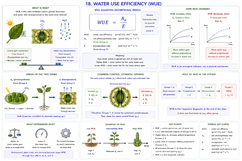
The image shows how this indicator integrates the two main currents that cross the system. On the one hand, atmospheric carbon appears that enters through the stomata and is transformed into biomass through photosynthesis. On the other hand, water absorbed from the soil ascends through the xylem and finally leaves the plant as vapor through the same stomata. Water use efficiency compares both processes, expressing how much carbon the plant manages to incorporate for each unit of water consumed. When biomass production increases without water loss increasing in the same proportion, the indicator improves. If, on the other hand, the plant loses large amounts of water to fix relatively little carbon, efficiency decreases.
From the physiological point of view, this indicator reflects the operating strategy adopted by the plant in the face of environmental conditions. A wide stomatal opening favors the entry of carbon dioxide and can increase photosynthesis, but simultaneously increases transpiration and the risk of cavitation. A more intense stomatal closure protects the hydraulic system and reduces water consumption, although it also limits the supply of carbon dioxide and decreases biomass production. As a consequence, water use efficiency does not increase simply by maximizing photosynthesis or minimizing transpiration, but by finding a balance between both processes.
This behavior highlights one of the fundamental principles of the model: the different physiological processes cannot be optimized independently because they share the same control variable, stomatal opening. Any modification aimed at improving one of the objectives inevitably affects the others. Increasing stomatal conductance favors carbon fixation, but also increases water loss and tension in the xylem. Reducing conductance decreases transpiration and protects the hydraulic system, but simultaneously limits carbon dioxide supply and photosynthetic productivity. Efficiency in water use precisely summarizes the final result of this structural commitment.
Within the integrated model, this equation constitutes the closure of the entire causal chain. It does not introduce new feedback or modify the behavior of previous processes, but instead synthesizes the overall performance of the system into a single value. All the mechanisms previously described, from water retention in the soil to carbon fixation in chloroplasts, finally converge in this indicator. Therefore, water use efficiency represents an integrated measure of the plant's ability to transform available water resources into plant growth, allowing different environmental conditions, physiological strategies or evolutionary adaptations to be compared using a single parameter that summarizes the complete functioning of the model.
ID:('gp', 646)
Palos Verdes, Costa de Corral, Región de los Rios, Chile