
In liquid column
Storyboard 
In the case of a column of liquid, Bernoulli's law can be applied along with the hydrostatic pressure term. However, it's important to note that when viscosity of the liquid is not considered, the reduction in level occurs uniformly. In this regard, it can be modeled using the continuity equation to determine the downward velocity of the cylinder.For a column of liquid with an outlet at the bottom, the behavior is similar to what is estimated with Bernoulli's principle. Differences arise due to the formation of small vortices at the outlet, effectively reducing the outlet area and obstructing the flow. However, the flow of a low-viscosity liquid can be modeled in the zone without vortices using Bernoulli's principle.
ID:(1427, 0)
Static and dynamic pressure
Description
When you have four columns with different cross-sections interconnected, the liquid will assume the same level in all of them. If you open the interconnecting channel, the liquid will start to flow towards the opening where the pressure is equal to the ambient pressure. In the first cylinder, the pressure is equal to the pressure of the water column plus the atmospheric pressure, so the difference with respect to the pressure at the exit is the pressure of the first column. The liquid begins to gain velocity while the dynamic pressure starts to decrease, which is evident in the increasingly smaller columns.

ID:(11092, 0)
Column emptying experiment
Description
This means that as the column empties and the height $h$ decreases, the velocity $v$ also decreases proportionally.
The key parameters are:• Inner diameter of the vessel: 93 mm• Inner diameter of the evacuation channel: 3 mm• Length of the evacuation channel: 18 mmThese parameters are important to understand and analyze the process of column emptying and how the exit velocity varies with height.
ID:(9870, 0)
In liquid column
Model
In the case of a column of liquid, Bernoulli's law can be applied along with the hydrostatic pressure term. However, it's important to note that when viscosity of the liquid is not considered, the reduction in level occurs uniformly. In this regard, it can be modeled using the continuity equation to determine the downward velocity of the cylinder. For a column of liquid with an outlet at the bottom, the behavior is similar to what is estimated with Bernoulli's principle. Differences arise due to the formation of small vortices at the outlet, effectively reducing the outlet area and obstructing the flow. However, the flow of a low-viscosity liquid can be modeled in the zone without vortices using Bernoulli's principle.
Variables
Calculations
Calculations
Equations
(ID 3469)
(ID 3804)
If there is the pressure difference ($\Delta p$) between two points, as determined by the equation:
| $ dp = p - p_0 $ |
we can utilize the water column pressure ($p$), which is defined as:
| $ p_t = p_0 + \rho_w g h $ |
This results in:
$\Delta p=p_2-p_1=p_0+\rho_wh_2g-p_0-\rho_wh_1g=\rho_w(h_2-h_1)g$
As the height difference ($\Delta h$) is:
| $ \Delta h = h_2 - h_1 $ |
the pressure difference ($\Delta p$) can be expressed as:
| $ \Delta p = \rho_w g \Delta h $ |
(ID 4345)
Using Bernoulli's equation, we can analyze the case of a column of water that generates a pressure difference:
| $ \Delta p = \rho_w g \Delta h $ |
and induces a velocity flow $v$ through a tube, in accordance with:
| $ \Delta p = - \rho \bar{v} \Delta v $ |
Thus, we can estimate the velocity as:
$v = \sqrt{2 g h}$
This velocity, through a tube section of radius $R$, results in a flow:
$J = \pi R^2 v$
If the column has a cross-sectional area $S$, and its height decreases with respect to the variation in height $h$ over time $t$, we can apply the law of continuity, which states:
| $ S_1 j_{s1} = S_2 j_{s2} $ |
Therefore, the equation that describes this situation is:
| $ S\displaystyle\frac{dh}{dt} = \pi R^2 \sqrt{2gh}$ |
(ID 9882)
If in the equation
| $ S\displaystyle\frac{dh}{dt} = \pi R^2 \sqrt{2gh}$ |
the constants are replaced by
| $ \tau_b = \displaystyle\frac{S}{\pi R^2}\sqrt{\displaystyle\frac{h_0}{g}}$ |
we obtain the first-order linear differential equation
$\displaystyle\frac{dh}{dt}=\displaystyle\frac{1}{\tau_b} \sqrt{h_0 h}$
whose solution is
| $ h = h_0\left(1-\displaystyle\frac{t}{\tau_b}\right)^2$ |
(ID 14524)
In this case, it can be assumed that the mean Speed of Fluid in Point 2 ($v_2$) represents zero velocity and the mean Speed of Fluid in Point 1 ($v_1$) corresponds to the flow speed ($v_s$). Therefore, for the speed difference between surfaces ($\Delta v$) the following is established:
$\Delta v = v_2 - v_1 = 0 - v_s = - v_s$
and for the average speed ($\bar{v}$) it is calculated:
$\bar{v} = \displaystyle\frac{v_1 + v_2}{2} = \frac{v_s}{2}$
Consequently, with the variación de la Presión ($\Delta p$), which equals the pressure difference ($\Delta p_s$), we obtain:
| $ \Delta p = - \rho \bar{v} \Delta v $ |
resulting in:
$\Delta p_s = \displaystyle\frac{1}{2} \rho v_s^2$
leading to:
| $ v_s = \sqrt{\displaystyle\frac{2 \Delta p_s }{ \rho }}$ |
(ID 15710)
The volume ($V$) for a tube with constant the section Tube ($S$) and a position ($s$) is
| $ V = h S $ |
If the section Tube ($S$) is constant, the temporal derivative will be
$\displaystyle\frac{dV}{dt} = S\displaystyle\frac{ds}{dt}$
thus, with the volume flow ($J_V$) defined by
| $ J_V =\displaystyle\frac{ dV }{ dt }$ |
and with the flux density ($j_s$) associated with the position ($s$) via
| $ j_s =\displaystyle\frac{ ds }{ dt }$ |
it is concluded that
| $ J_V = S j_s $ |
(ID 15716)
Examples
(ID 15487)
If there is a column height ($h$) of liquid with the liquid density ($\rho_w$) under the effect of gravity, using the gravitational Acceleration ($g$), the variación de la Presión ($\Delta p$) is generated according to:
| $ \Delta p = \rho_w g \Delta h $ |
This the variación de la Presión ($\Delta p$) produces a flow through the outlet tube with the tube length ($\Delta L$), the tube radius ($R$), and the viscosity ($\eta$) of a volume flow 1 ($J_{V1}$) according to the Hagen-Poiseuille law:
| $ J_V =-\displaystyle\frac{ \pi R ^4}{8 \eta }\displaystyle\frac{ \Delta p }{ \Delta L }$ |
Since this equation includes the section in point 2 ($S_2$), the flux density 2 ($j_{s2}$) can be calculated using:
| $ j_s = \displaystyle\frac{ J_V }{ S }$ |
With this, we obtain:
| $ j_s = \displaystyle\frac{ \rho_w g R ^2}{8 \eta \Delta L } h $ |
which corresponds to an average velocity.
To model the system, the key parameters are:• Interior diameter of the container: 93 mm• Interior diameter of the evacuation channel: 3.2 mm• Length of the evacuation channel: 18 mmThe initial liquid height is 25 cm.
(ID 11092)
Let's consider the system of a cylindrical bucket with a drainage hole. When the plug is removed, the water starts to flow due to the existing pressure. According to Bernoulli's principle, inside the bucket ($v\sim 0$), the velocity is zero, and we have:
$\displaystyle\frac{1}{2}\rho v^2 + \rho g h\sim \rho g h$
while outside the bucket ($h=0$), only the kinetic component exists:
$\displaystyle\frac{1}{2}\rho v^2 + \rho g h\sim \displaystyle\frac{1}{2}\rho v^2$
Since both expressions are equal, we have:
$\displaystyle\frac{1}{2}\rho v^2=\rho g h$
which gives the velocity as:
$v=\sqrt{2 g h}$
To compare with the experiment, we can use this expression to estimate, with:
| $ S\displaystyle\frac{dh}{dt} = \pi R^2 \sqrt{2gh}$ |
the range that the stream should have. If we plot it graphically, we observe:
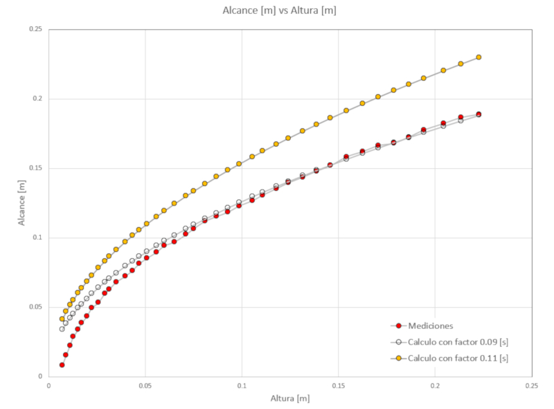
where:• the red dots correspond to the experimental measurements,• the blue dots correspond to the calculated range using a factor of 0.11,• the transparent dots correspond to the calculated range using a factor of 0.09.Therefore, we can conclude that Bernoulli's model overestimates the velocity at which the bucket empties. This is because in the vicinity of the drainage hole, the effects of viscosity are not negligible, and therefore, the velocity is lower.
(ID 11063)
If the Tracker program is used, the height of the meniscus of the column and the range of the jet can be measured. The relationship between the two is shown in the following graph:
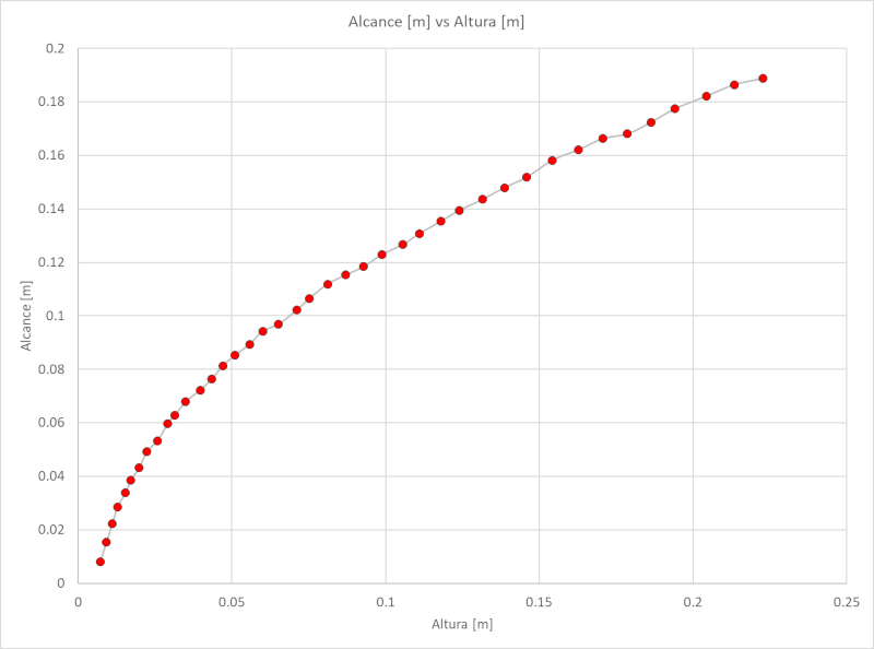
Reach [m] vs Height [m]
The recorded data, which can be downloaded as an Excel table from the following link excel table, are as follows:
| Time [s] | Height [m] | Reach [m] |
| 0 | 2.23E-01 | 1.89E-01 |
| 4 | 2.14E-01 | 1.86E-01 |
| 8 | 2.04E-01 | 1.82E-01 |
| 12 | 1.94E-01 | 1.77E-01 |
| 16 | 1.86E-01 | 1.72E-01 |
| 20 | 1.79E-01 | 1.68E-01 |
| 24 | 1.71E-01 | 1.66E-01 |
| 28 | 1.63E-01 | 1.62E-01 |
| 32 | 1.54E-01 | 1.58E-01 |
| 36 | 1.46E-01 | 1.52E-01 |
| 40 | 1.39E-01 | 1.48E-01 |
| 44 | 1.32E-01 | 1.44E-01 |
| 48 | 1.24E-01 | 1.39E-01 |
| 52 | 1.18E-01 | 1.35E-01 |
| 56 | 1.11E-01 | 1.31E-01 |
| 60 | 1.06E-01 | 1.27E-01 |
| 64 | 9.88E-02 | 1.23E-01 |
| 68 | 9.29E-02 | 1.18E-01 |
| 72 | 8.70E-02 | 1.15E-01 |
| 76 | 8.11E-02 | 1.12E-01 |
| 80 | 7.52E-02 | 1.06E-01 |
| 84 | 7.12E-02 | 1.02E-01 |
| 88 | 6.51E-02 | 9.69E-02 |
| 92 | 6.00E-02 | 9.42E-02 |
| 96 | 5.58E-02 | 8.94E-02 |
| 100 | 5.09E-02 | 8.52E-02 |
| 104 | 4.70E-02 | 8.13E-02 |
| 108 | 4.34E-02 | 7.63E-02 |
| 112 | 3.97E-02 | 7.22E-02 |
| 116 | 3.49E-02 | 6.79E-02 |
| 120 | 3.15E-02 | 6.28E-02 |
| 124 | 2.91E-02 | 5.96E-02 |
| 128 | 2.58E-02 | 5.33E-02 |
| 132 | 2.23E-02 | 4.92E-02 |
| 136 | 1.98E-02 | 4.31E-02 |
| 140 | 1.71E-02 | 3.85E-02 |
| 144 | 1.54E-02 | 3.38E-02 |
| 148 | 1.28E-02 | 2.85E-02 |
| 152 | 1.11E-02 | 2.23E-02 |
| 156 | 9.17E-03 | 1.54E-02 |
| 160 | 7.15E-03 | 7.95E-03 |
(ID 11062)
(ID 15490)
ID:(1427, 0)