Build linear model with estimator (Titanic dataset)
Storyboard 
One application is the study of the data of the passengers of the Titanic and the probability of survival according to their characteristics. In this case, a model of a linear estimator type is used.
Code and data
ID:(1790, 0)
Setup for linear model
Description 
Setup for linear model:
import os
import sys

import numpy as np
import pandas as pd
import matplotlib.pyplot as plt
from IPython.display import clear_output
from six.moves import urllib
ID:(13828, 0)
Load dataset
Description 
Load the passenger data for the maiden voyage of the Titanic:
import tensorflow.compat.v2.feature_column as fc
import tensorflow as tf

# Load dataset.
dftrain = pd.read_csv('titanic_lin_train.csv')
dfeval = pd.read_csv('titanic_lin_eval.csv')
dftest = pd.read_csv('titanic_lin_test.csv')
y_train = dftrain.pop('survived')
y_eval = dfeval.pop('survived')
ID:(13829, 0)
Show structures and data
Description 
Show structures and data from the Titanic passenger dataset:
# show structure and data
dftrain.head()

ID:(13830, 0)
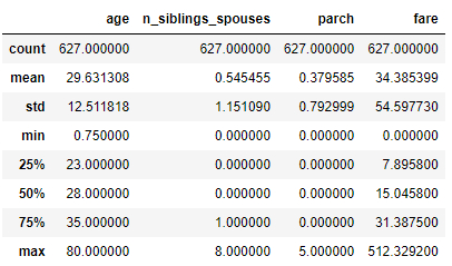
Show Data Statistics
Description 
Show Titanic Passenger Data Statistics
# show statistics of data
dftrain.describe()
ID:(13831, 0)
Number of records to train and evaluate
Description 
Number of records to train and evaluate:
# number of train and evaluation records
dftrain.shape[0], dfeval.shape[0]
(627, 264)
ID:(13832, 0)
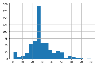
Show the histogram (vertical) of the age
Description 
To show the histogram (vertical) hist of the ages dftrain.age with interval of 20 years (bins = 20) is obtained from
# age histogram
dftrain.age.hist(bins=20)
ID:(13833, 0)
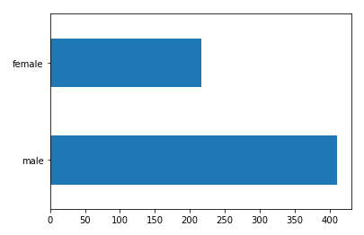
Show the histogram (horizontal) of the gender
Description 
To show the histogram (horizontal) plot (kind = 'barh') of the gender dftrain.sex counting the number of passengers according to gender value_counts () you get# gender histogram
dftrain.sex.value_counts().plot(kind='barh')
ID:(13834, 0)
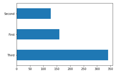
Show the histogram (horizontal) of the classes
Description 
To show the histogram (horizontal) plot (kind='barh') of the class dftrain['class'] counting the number of passengers according to class value_counts () you get
# class histogram
dftrain['class'].value_counts().plot(kind='barh')
ID:(13835, 0)
Show the histogram (horizontal) of the classes
Description 
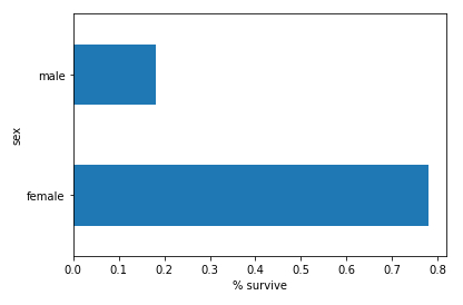
To show the histogram (horizontal) plot(kind='barh') of the survivors survived averaged mean() grouped by gender groupby('sex') with the label on the x-axis set_xlabel('% survive') of the string assembled by concatenating pd.concat([dftrain, y_train], axis = 1) of all the data dftrain and the abscissa y_train;
# survived histogram
pd.concat([dftrain, y_train], axis=1).groupby('sex').survived.mean().plot(kind='barh').set_xlabel('% survive')
ID:(13836, 0)
Form columns of data
Description 
To form the tensor, the feature_columns data must be added according to whether they are categories or numeric.
The former are rescued via the vocabulary array and added with the append command, forming the column with the tf.feature_column.categorical_column_with_vocabulary_list command.
The latter are assigned directly with the append command with the column via its tf.feature_column.numeric_column designation.
# define tensor
feature_columns = []

# define categorical columns names
CATEGORICAL_COLUMNS = ['sex', 'class', 'deck', 'embark_town', 'alone']
# build columns of categorical variables
for feature_name in CATEGORICAL_COLUMNS:
  vocabulary = dftrain[feature_name].unique()
  feature_columns.append(tf.feature_column.categorical_column_with_vocabulary_list(feature_name, vocabulary))

# define numeric columns names
FLOAT_COLUMNS = ['age', 'fare']
# build columns of numeric variables
for feature_name in FLOAT_COLUMNS:
  feature_columns.append(tf.feature_column.numeric_column(feature_name, dtype=tf.float32))

# define numeric columns names
NUMERIC_COLUMNS = ['n_siblings_spouses', 'parch']
# build columns of numeric variables
for feature_name in NUMERIC_COLUMNS:
  feature_columns.append(tf.feature_column.numeric_column(feature_name, dtype=tf.int32))
ID:(13837, 0)
Form set to train and evaluate
Description 
A function is defined to generate arrangements for the training and evaluation processes:
# define function for making set
def make_input_fn(data_df, label_df, num_epochs=10, shuffle=True, batch_size=32):
  def input_function():
    ds = tf.data.Dataset.from_tensor_slices((dict(data_df), label_df))
    if shuffle:
      ds = ds.shuffle(1000)
    ds = ds.batch(batch_size).repeat(num_epochs)
    return ds
  return input_function
Generation of sets for training and evaluation:
# generate training input
train_input_fn = make_input_fn(dftrain, y_train)
# generate evaluating input
eval_input_fn = make_input_fn(dfeval, y_eval, num_epochs=1, shuffle=False)
ID:(13838, 0)
Training and Evaluation
Description 
To perform the classification, the model is defined using the estimator.LinearClassifier function applied to the columns of the feature_columns data.
# define model
linear_model = tf.estimator.LinearClassifier(feature_columns=feature_columns)
Then we proceed to train the model by applying train on the model linear_model with the data to train train_input_fn
# define train model
linear_model.train(train_input_fn)
Finally it is evaluated with evaluate applied on the model linear_model and the data to evaluate eval_input_fn
# evaluate model
result = linear_model.evaluate(eval_input_fn)
El resultado final se imprime en mediante el comando print:
# print result
clear_output()
print(result)
Is obtained:
{'accuracy': 0.75757575, 'accuracy_baseline': 0.625, 'auc': 0.83067036, 'auc_precision_recall': 0.78773487, 'average_loss': 0.49594572, 'label/mean': 0.375, 'loss': 0.49112648, 'precision': 0.65217394, 'prediction/mean': 0.44832677, 'recall': 0.75757575, 'global_step': 200}
ID:(13841, 0)
Histogram of the probabilities of survival
Description 
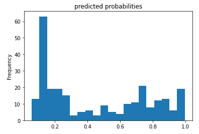
If the predicted probability of survival is evaluated based on its frequency:
# histogram of the probability
pred_dicts = list(linear_est.predict(eval_input_fn))
probs = pd.Series([pred['probabilities'][1] for pred in pred_dicts])

probs.plot(kind='hist', bins=20, title='predicted probabilities')
a distribution of the form is obtained:
ID:(13839, 0)
ROC Curve
Description 
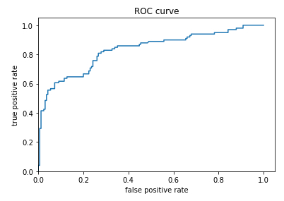
To use this forecast, a limit value of the property must be defined to define on which value the survival will be predicted and under which the non-survival will be forecast. To do this, the probability that survival is predicted and observed (true positive) must be evaluated and compared with the probability that survival is predicted when it is not survived (false positive).\\nThe true-positive
$TPR=\displaystyle\frac{TP}{TP+FN}$
\\n\\nwhere true-positive
$FPR=\displaystyle\frac{FP}{FP+TN}$
where false-positive
from sklearn.metrics import roc_curve
from matplotlib import pyplot as plt

fpr, tpr, _ = roc_curve(y_eval, probs)
plt.plot(fpr, tpr)
plt.title('ROC curve')
plt.xlabel('false positive rate')
plt.ylabel('true positive rate')
plt.xlim(0,)
plt.ylim(0,)
The representation of both probabilities is called a ROC (Receiver Operating Characteristic) diagram:
ID:(13840, 0)
