SARS 2003 epidemic in Hong Kong
Image
In 2003 there is an outbreak of SARS (Severe acute respiratory syndrome) in China that spreads to Hong Kong and then to the entire world. The following map shows the number of cases in the different countries:

ID:(9662, 0)
SARS simulator - adjustment of a SEIR Model
Php
This simulator contains the SARS epidemic data for the case of Hong Kong and allows searching the parameters of a SEIR model by adjusting the curves to the actual values:
ID:(9659, 0)
SARS 2003 epidemic analysis in Hong Kong
Image
If the WHO data for the SARS epidemic in 2003 in Hong Kong is studied, the current number of infected

\\n\\nEven if you do not have the beginning section, you can see the maximum typical of the number of infected when you start to control them and it is given that\\n\\n
$\displaystyle\frac{dS}{dt}=\left(\displaystyle\frac{\beta C}{N}S-\gamma\right)I=0$
\\n\\nso that those susceptible at that point reach\\n\\n
$S=\displaystyle\frac{\gamma}{\beta C}N$
ID:(8202, 0)
2003 SARS Parameter Determination in Hong Kong
Image
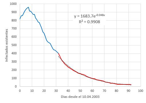
If you study the way in which the infected descend, it is seen that as time progresses, the term gamma must dominate since it is the one that reduces the total volume described by the first term. That is why it is necessary for times when the epidemic is under control\\n\\n
$\displaystyle\frac{dI}{dt}=\left(\displaystyle\frac{\beta C}{N}S-\gamma\right)I\sim-\gamma I$
\\n\\nIn that case the asymptomatic solution is of the form\\n\\n
$I(t) \propto e^{-\gamma t}$
what can be seen in the existing infected curve for the SARS 2003 case in Hong Kong. Therefore, a minimum square adjustment of the final part of the curve can be made

\\n\\nobtaining that the factor
$\tau=\displaystyle\frac{1}{\gamma}\sim 20.8,dias$
If we also assume that each person meets on a daily basis with the order of 30 people, the
ID:(8203, 0)
SIR model to describe SARS 2003 in Hong Kong
Image
If the susceptible, infected and 'recovered' (who heal or die) are observed, the typical curves of the SIR model are observed:

ID:(9663, 0)
Adjusted data
Image
If the contagion and development parameters are varied, the sums of:
• the infected
• the recovered
• the dead
As the following picture shows:

ID:(9693, 0)
Effect of increasing N
Image
If the number of people belonging to the group in which the disease is spread is very large, the curve tends to exceed the measured data:

ID:(9694, 0)
Effect of reducing N
Image
If the number of people belonging to the group in which the disease is spread is very small, the curve tends to exceed the measured data:

ID:(9695, 0)
Effect of increasing $\beta C$
Image
If the number of contacts and the rate of infection is too large the slope is too large (very steep):

ID:(9696, 0)
Effect of reducing $\beta C$
Image
If the number of contacts and the rate of infection is too small, the slope is too small (too flat):

ID:(9697, 0)
Time lag
Description
The delay time allows the curve to be moved by transporting it without deformation along the time axis. It is necessary since the time in which the disease has started is unknown and exists for each of the curves individually.\\n\\nEach curve moves individually in the times:\\n\\n• $t_{\rho}$ time when the first latent appears\\n• $t_{\beta}$ time when the first infected appears\\n• $t_{\gamma}$ time when the first recovered appears\\n• $t_{\delta}$ time at which the first dead appears\\n\\nIn general it should be that the times are such that\\n\\n
$t_{\rho} < t_{\beta} < t_{\gamma} < t_{\delta}$
given the sequence of events in the model. However, the adjustment and uncertainty in the data can give different orders that indicate that the times themselves are not reliable.
Important is to recognize that the offset can be both positive and negative.
ID:(9702, 0)
Very large delay time effect, example of infection
Image
If the delay time of each curve is chosen too large the curve is delayed with respect to the real evolution:

ID:(9698, 0)
Effect of delay time too small, example of infection
Image
If the delay time of each curve is chosen too small, the curve moves forward with respect to the actual evolution:

ID:(9699, 0)
Effect of recovery rate and/or latency term
Image
If the recovery rate and the latency rate are too large, the infected curve becomes steeper while the recovery rate flattens. In that sense, these factors seem to rotate both curves increasing (if they grow) and decreasing (if they decrease) the angle between them.

ID:(9700, 0)
Death rate effect
Image
If the death rate grows the corresponding curve has a greater participation in the population that no longer infects and is generically called 'recovered':

ID:(9701, 0)
