Build DNN model with estimator (Titanic dataset)
Storyboard 
One application is the study of the data of the passengers of the Titanic and the probability of survival according to their characteristics. In this case, a model of the DNN class estimator type is used.
Code and data
ID:(1791, 0)
Load dataset
Description 
Load the passenger data for the maiden voyage of the Titanic:
import pandas as pd
import numpy as np

train = pd.read_csv('train_short.csv')
eval = pd.read_csv('eval_short.csv')
test = pd.read_csv('test-ready.csv')
ID:(13843, 0)
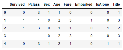
Show structures and data for training
Description 
Show structures and data from the Titanic passenger dataset:
# show structure and data
train.head(5)
ID:(13844, 0)
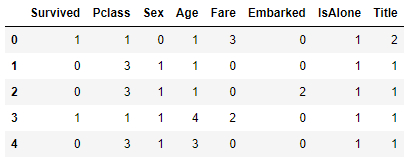
Show structures and data for evaluation
Description 
Show structures and data from the Titanic passenger dataset:
# show structure and data
eval.head(5)
ID:(13845, 0)
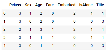
Show structures and data for test
Description 
Show structures and data from the Titanic passenger dataset:
# show structure and data
test.head(5)
ID:(13846, 0)
Number of records
Description 
The number of records for each group can be determined with the shape[0] function:
# count number of records
train.shape[0], eval.shape[0], test.shape[0]
(627, 264, 418)
ID:(13847, 0)
Upload data to train and evaluate
Description 
In order to run the training, you must load the data from both training train_input_fn and evaluation eval_input_fn in tensors and shuffle them:
# input function for training
def train_input_fn(features, labels, batch_size):
    dataset = tf.data.Dataset.from_tensor_slices((dict(features), labels))
    dataset = dataset.shuffle(10).repeat().batch(batch_size)
    return dataset

# input function for evaluation or prediction
def eval_input_fn(features, labels, batch_size):
    features=dict(features)
    if labels is None:
        inputs = features
    else:
        inputs = (features, labels)

    dataset = tf.data.Dataset.from_tensor_slices(inputs)

    assert batch_size is not None, 'batch_size must not be None'
    dataset = dataset.batch(batch_size)

    return dataset
ID:(13848, 0)
Form arrangements train and evaluate
Description 
Create arrays of base and variable data to predict to train and evaluate. In this case the column to be predicted is survival, which is obtained by pop('Survived'):
# define training arrays
y_train = train.pop('Survived')
X_train = train

# define evaluation arrays
y_eval = eval.pop('Survived')
X_eval = eval
ID:(13849, 0)
Create array of columns to define model
Description 
To define the model, the arrangement of the columns feature_columns is created that will be used by:
# import tensorflow
import tensorflow as tf

# define columns
feature_columns = []

for key in X_train.keys():
    feature_columns.append(tf.feature_column.numeric_column(key=key))
ID:(13850, 0)
Define the DNN model
Description 
With the feature_columns columns you can define the DNN_model model with estimator.DNNClassifier:
# define the DNN model
DNN_model = tf.estimator.DNNClassifier(
    feature_columns=feature_columns,
    hidden_units=[10, 10],
    n_classes=2)
ID:(13851, 0)
Train the DNN model
Description 
Train the model with the data created by train_input_fn:
# train the DNN model
batch_size = 100
train_steps = 400

for i in range(0,100):
    DNN_model.train(input_fn=lambda:train_input_fn(X_train, y_train,batch_size),steps=train_steps)
INFO:tensorflow:Calling model_fn.
INFO:tensorflow:Done calling model_fn.
INFO:tensorflow:Create CheckpointSaverHook.
INFO:tensorflow:Graph was finalized.
INFO:tensorflow:Running local_init_op.
INFO:tensorflow:Done running local_init_op.
INFO:tensorflow:Calling checkpoint listeners before saving checkpoint 0...
INFO:tensorflow:Saving checkpoints for 0 into C:\Users\KLAUSS~1\AppData\Local\Temp\tmp9f9txo1c\model.ckpt.
INFO:tensorflow:Calling checkpoint listeners after saving checkpoint 0...
INFO:tensorflow:loss = 0.6394816, step = 0
INFO:tensorflow:global_step/sec: 807.462
INFO:tensorflow:loss = 0.60958487, step = 100 (0.125 sec)
INFO:tensorflow:global_step/sec: 1143.95
INFO:tensorflow:loss = 0.6261593, step = 200 (0.086 sec)
INFO:tensorflow:global_step/sec: 1233.15
INFO:tensorflow:loss = 0.58592194, step = 300 (0.081 sec)
...
INFO:tensorflow:Calling checkpoint listeners before saving checkpoint 40000...
INFO:tensorflow:Saving checkpoints for 40000 into C:\Users\KLAUSS~1\AppData\Local\Temp\tmp9f9txo1c\model.ckpt.
INFO:tensorflow:Calling checkpoint listeners after saving checkpoint 40000...
INFO:tensorflow:Loss for final step: 0.49167815.
ID:(13852, 0)
Evaluate the DNN model
Description 
Evaluate the model with the data created by eval_input_fn:
# evaluate the DNN model
eval_result = DNN_model.evaluate(input_fn=lambda:eval_input_fn(X_eval, y_eval,batch_size))
INFO:tensorflow:Calling model_fn.
INFO:tensorflow:Done calling model_fn.
INFO:tensorflow:Starting evaluation at 2021-07-26T22:14:15
INFO:tensorflow:Graph was finalized.
INFO:tensorflow:Restoring parameters from C:\Users\KLAUSS~1\AppData\Local\Temp\tmp9f9txo1c\model.ckpt-40000
INFO:tensorflow:Running local_init_op.
INFO:tensorflow:Done running local_init_op.
INFO:tensorflow:Inference Time : 0.36007s
INFO:tensorflow:Finished evaluation at 2021-07-26-22:14:15
INFO:tensorflow:Saving dict for global step 40000: accuracy = 0.7765151, accuracy_baseline = 0.6363636, auc = 0.8616692, auc_precision_recall = 0.80749995, average_loss = 0.44881073, global_step = 40000, label/mean = 0.36363637, loss = 0.44580325, precision = 0.7078652, prediction/mean = 0.36897483, recall = 0.65625
INFO:tensorflow:Saving 'checkpoint_path' summary for global step 40000: C:\Users\KLAUSS~1\AppData\Local\Temp\tmp9f9txo1c\model.ckpt-40000
ID:(13853, 0)
Perform forecast with the DNN model
Description 
Forecast the model output with the evaluation data created by eval_input_fn:
# forcast with the DNN model
predictions = DNN_model.predict(
    input_fn=lambda:eval_input_fn(eval,labels=None,
    batch_size=batch_size))

results = list(predictions)
INFO:tensorflow:Calling model_fn.
INFO:tensorflow:Done calling model_fn.
INFO:tensorflow:Graph was finalized.
INFO:tensorflow:Restoring parameters from C:\Users\KLAUSS~1\AppData\Local\Temp\tmp9f9txo1c\model.ckpt-40000
INFO:tensorflow:Running local_init_op.
INFO:tensorflow:Done running local_init_op.
ID:(13854, 0)
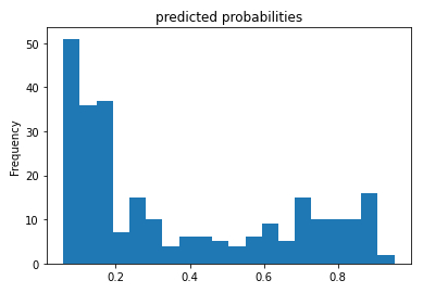
Histogram of the probabilities of survival
Description 
If the predicted probability of survival is evaluated based on its frequency:
# histogram of the probability
probs = pd.Series([pred['probabilities'][1] for pred in results])

probs.plot(kind='hist', bins=20, title='predicted probabilities')
a distribution of the form is obtained:
ID:(13855, 0)
ROC Curve
Description 
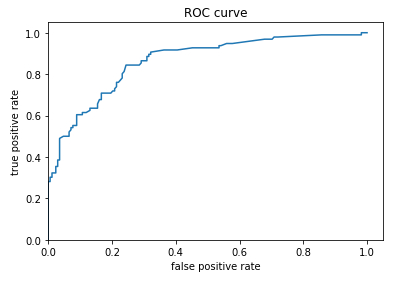
To use this forecast, a limit value of the property must be defined to define on which value the survival will be predicted and under which the non-survival will be forecast. To do this, the probability that survival is predicted and observed (true positive) must be evaluated and compared with the probability that survival is predicted when it is not survived (false positive).\\nThe true-positive
$TPR=\displaystyle\frac{TP}{TP+FN}$
\\n\\nwhere true-positive
$FPR=\displaystyle\frac{FP}{FP+TN}$
where false-positive
from sklearn.metrics import roc_curve
from matplotlib import pyplot as plt

fpr, tpr, _ = roc_curve(y_eval, probs)
plt.plot(fpr, tpr)
plt.title('ROC curve')
plt.xlabel('false positive rate')
plt.ylabel('true positive rate')
plt.xlim(0,)
plt.ylim(0,)
The representation of both probabilities is called a ROC (Receiver Operating Characteristic) diagram:
ID:(13842, 0)
